11  Subcriteria A2b

Using R with terra package

11.1 Updating the assessment workflow

The original workflow included a combination of two remote sensing products (Friedl et al. 2010; Hansen et al. 2013). The updated workflow is based on an updated version of one data source that spans more years and uses improved algorithms. We have two version of the workflow, one based on R and local copies of the remote sensing products (this chapter), and one based on Python and Earth Engine for cloud computing (see Section 12.1).

Differences between original and updated assessment workflows for subcriterion A2b.

Step	2019	2025 (R)	2025 (Python)
GIS data prep.	GRASS GIS / gdal / R	R / gdal / terra	Earth Engine
Data source	GFC v1.2 (2015) and MODIS LC v5.1	GFC v1.12 (2024)	GFC v1.12 (2024)
Analysis	R / glm	R / glm / redlistr	Python / Earth Engine
Timeframe	2000-2050	2000-2050	2000-2050

11.2 Set up

Load packages

We will run this analysis using the following packages in R.

suppressPackageStartupMessages({
    library(terra)
    library(sf)
    library(dplyr)
    library(tidyr)
    library(units)
    library(exactextractr)
    library(redlistr)
    })

Load data

We start by configuring the relative path to our data folder:

here::i_am("R/subcriterion-A2b.ipynb")
data_dir <- here::here("downloaded-data")

here() starts at /Users/z3529065/proyectos/Forests-Americas/RLE-example-dry-forest-guajira

We already downloaded the vector data for the distribution of the target macrogroup from OSF in Chapter 4, now we read the spatial data in vector format using the function vect from package terra:

M563 <- read_sf(here::here(data_dir,
  "1.A.1.Ei.563---Guajiran-Seasonal-Dry-Forest-1km.gpkg"))

We already downloaded and prepared the GFC data for estimates of tree cover in Chapter 7, now we read the spatial data in raster format using the function rast from package terra.

tif_files <- dir(
  here::here(data_dir,"GFC-2024-v1.12"), 
  recursive=TRUE, 
  pattern="*tif$",
  full.names=TRUE)

lossyear <- rast( grep("lossyear", tif_files, value=TRUE)) 
gain <- rast(grep("gain", tif_files, value=TRUE)) 
cover <- rast(grep("treecover2000", tif_files, value=TRUE)) 
cover24 <- rast(grep("treecover2024", tif_files, value=TRUE)) 

A quick check that this is indeed correct:

plot(cover)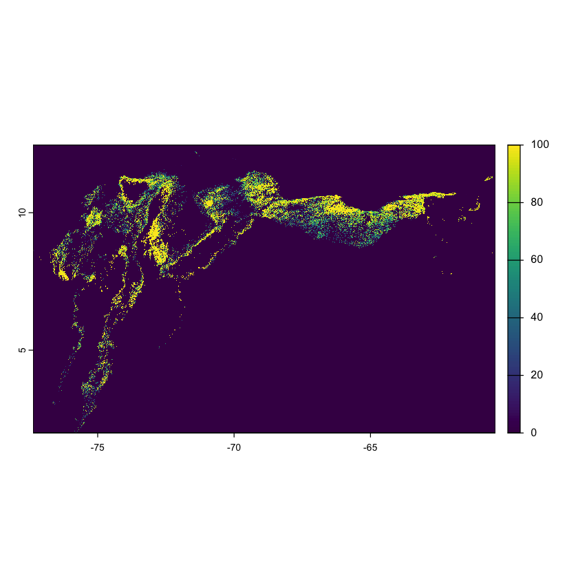

Now make a couple of extra files for the calculations below:

loss <- (lossyear > 0) + 0
initial <- (cover > 0) + 0

Now we bundle these raster files together:

gfc <- c(cover, cover24, initial, gain, loss)
names(gfc) <- c("cover00", "cover24", "initial", "gain", "loss")

The data is in unprojected units, but we can calculate the resolution for each cell:

raster_resolution <- cellSize(loss)

raster_resolution

class       : SpatRaster 
size        : 41880, 67800, 1  (nrow, ncol, nlyr)
resolution  : 0.00025, 0.00025  (x, y)
extent      : -77.37, -60.42, 1.99, 12.46  (xmin, xmax, ymin, ymax)
coord. ref. : lon/lat WGS 84 (EPSG:4326) 
source      : spat_102fafb106af_66298_P2mm2aa9P9QX7pk.tif 
varname     : GFC-2024-v1.12.M563.lossyear 
name        :     area 
min value   : 751.6660 
max value   : 768.8654 

11.3 Summarise changes

Processing these large raster files in R can be slow, but it is possible to speed up the calculations by using a grid and functions from library exactextractr:

rawgrid <- st_make_grid(M563, cellsize = .091)
grid <- st_sf(id = 1:length(rawgrid), geoms = rawgrid, 
        stringsAsFactors = FALSE)

We try with a cell size that is roughly 10 by 10 km in area:

range(set_units(st_area(grid),'km2'))

Units: [km^2]
[1]  99.99352 102.32401

Ok let’s run this while we get a cup of coffee or glass of water…

qry <- exact_extract(gfc, grid, fun="sum", append_cols = c("id"))

Cannot preload entire working area of 14178211740 cells with max_cells_in_memory = 3e+07. Raster values will be read for each feature individually.

  |======================================================================| 100%

res_gfc <- exact_extract(raster_resolution, grid, fun="mean", append_cols = c("id"),force_df=TRUE)

Cannot preload entire working area of 2835642348 cells with max_cells_in_memory = 3e+07. Raster values will be read for each feature individually.

  |======================================================================| 100%

Ok, we are back and we have some results, now we will try to summarise these per cell.

res_gfc <- res_gfc |> mutate(res=set_units(mean,'m2') |> set_units('km2'))

extent_estimates <- 
    tibble(qry) |> left_join(res_gfc,by='id') |>
        filter(sum.initial>0 | sum.gain>0) |>
        mutate(cells_2000=sum.initial,
               cells_2024=sum.initial + sum.gain - sum.loss,
               
               mean_2000 = (sum.cover00 / 100) / sum.initial,
               eco_extent_2000 = cells_2000 * res * mean_2000,
               eco_extent_2024 = cells_2024 * res * mean_2000,
               alt_extent_2000 = (sum.cover00/100) * res,
               alt_extent_2024 = (sum.cover24/100) * res
              )

head(extent_estimates)

A tibble: 6 × 15

id	sum.cover00	sum.cover24	sum.initial	sum.gain	sum.loss	mean	res	cells_2000	cells_2024	mean_2000	eco_extent_2000	eco_extent_2024	alt_extent_2000	alt_extent_2024
<int>	<dbl>	<dbl>	<dbl>	<dbl>	<dbl>	<dbl>	<[km^2]>	<dbl>	<dbl>	<dbl>	<[km^2]>	<[km^2]>	<[km^2]>	<[km^2]>
16	394338.00	368003.00	6402.000	9	367.00000	768.8402	0.0007688402 [km^2]	6402.000	6044.000	0.6159606	3.0318291 [km^2]	2.8622891 [km^2]	3.0318291 [km^2]	2.8293550 [km^2]
17	210969.00	187326.00	4873.000	1	404.00000	768.8402	0.0007688402 [km^2]	4873.000	4470.000	0.4329345	1.6220145 [km^2]	1.4878729 [km^2]	1.6220145 [km^2]	1.4402376 [km^2]
18	786993.69	704305.69	13946.496	59	1257.00000	768.8402	0.0007688402 [km^2]	13946.496	12748.496	0.5642949	6.0507239 [km^2]	5.5309685 [km^2]	6.0507239 [km^2]	5.4149853 [km^2]
19	69479.45	65038.04	1124.920	1	54.67097	768.8402	0.0007688402 [km^2]	1124.920	1071.249	0.6176392	0.5341859 [km^2]	0.5086994 [km^2]	0.5341859 [km^2]	0.5000386 [km^2]
205	336483.91	290286.06	5995.497	3	680.13544	768.7968	0.0007687968 [km^2]	5995.497	5318.361	0.5612278	2.5868776 [km^2]	2.2947139 [km^2]	2.5868776 [km^2]	2.2317100 [km^2]
206	873585.75	764134.00	16832.078	63	1703.53223	768.7968	0.0007687968 [km^2]	16832.078	15191.546	0.5190005	6.7160994 [km^2]	6.0615173 [km^2]	6.7160994 [km^2]	5.8746378 [km^2]

extent_estimates |> 
    summarise(
        raw2000=sum(alt_extent_2000),
        raw2024=sum(alt_extent_2024),
        eco2000=sum(eco_extent_2000, na.rm = TRUE), 
        eco2024=sum(eco_extent_2024, na.rm = TRUE))

A tibble: 1 × 4

raw2000	raw2024	eco2000	eco2024
<[km^2]>	<[km^2]>	<[km^2]>	<[km^2]>
97390.84 [km^2]	85126.09 [km^2]	97390.84 [km^2]	84968.26 [km^2]

11.4 Calculate declines

calc_decline <- function(data,start,end) {
  stopifnot("eco_extent" %in% colnames(data),
            "years" %in% colnames(data),
            start<=nrow(data),
            end<=nrow(data))
  start_date <- pull(data[start,"years"])
  end_date <- pull(data[end,"years"])
  stopifnot(start_date<end_date)
  start_extent <- pull(data[start,"eco_extent"])
  end_extent <- pull(data[end,"eco_extent"])
  res <- dplyr::tibble(
    start_date,
    end_date,
    time_frame = end_date-start_date,
    decline = (units::set_units(1,'1') - 
                 (end_extent/start_extent)) %>% 
      units::set_units('%')
      )
  if ("error_extent" %in% colnames(data)) {
    start_error <- pull(data[start,"error_extent"])
    end_error <- pull(data[end,"error_extent"])
    res$error <- sqrt(((end_extent^2 * start_error^2) + (start_extent^2 * end_error^2)) / (start_extent^4)) %>% units::set_units('%')
  }
  return(res)
}

rslts <- extent_estimates |> 
    dplyr::select(id,eco_extent_2000,eco_extent_2024) |>
    pivot_longer(c(eco_extent_2000,eco_extent_2024), 
                 names_prefix = "eco_extent_",
                 names_transform = as.numeric,
                 names_to = "years", values_to="eco_extent") |>
    group_by(years) |>
    summarise(eco_extent=sum(eco_extent, na.rm = TRUE))

rslts

A tibble: 2 × 2

years	eco_extent
<dbl>	<[km^2]>
2000	97390.84 [km^2]
2024	84968.26 [km^2]

85126.09 / 97390.84 

0.874066698675153

DS <- getDeclineStats(drop_units(rslts$eco_extent[1]), drop_units(rslts$eco_extent[2]), 
                           year.t1 = rslts$years[1], year.t2 = rslts$years[2],
                                 methods = c('PRD', 'ARD', 'ARC'))

DS

A data.frame: 1 × 4

absolute.loss	ARD	PRD	ARC
<dbl>	<dbl>	<dbl>	<dbl>
12422.58	517.6075	0.5669467	-0.56856

y_future <- extrapolateEstimate(drop_units(rslts$eco_extent[1]),  
                    year.t1 = rslts$years[1], 
                    nYears = 50,
                                  PRD = DS$PRD,
                                  ARD = DS$ARD,
                                  ARC = DS$ARC) |>
    tibble()

y_future

A tibble: 1 × 4

forecast.year	A.ARD.t3	A.PRD.t3	A.ARC.t3
<dbl>	<dbl>	<dbl>	<dbl>
2050	71510.46	73292.05	73292.05

rslts <- bind_rows(
    rslts,
    {transmute(y_future,
        eco_extent=set_units(A.ARD.t3,'km2'), 
        years=forecast.year) },
    {transmute(y_future,
        eco_extent=set_units(A.PRD.t3,'km2'), 
        years=forecast.year) },
    {transmute(y_future,
        eco_extent=set_units(A.ARC.t3,'km2'), 
        years=forecast.year) })

calc_decline(rslts,1,2:5)

A tibble: 4 × 4

start_date	end_date	time_frame	decline
<dbl>	<dbl>	<dbl>	<[%]>
2000	2024	24	12.75539 [%]
2000	2050	50	26.57373 [%]
2000	2050	50	24.74441 [%]
2000	2050	50	24.74441 [%]

st_area(M563) |> set_units('km2')

253656.4 [km^2]

(st_area(M563) |> set_units('km2') / (105206342 + 54502069 + 233854))

0.001585924 [km^2]

97390.84 /1.5

64927.2266666667

Friedl, Mark A., Damien Sulla-Menashe, Bin Tan, Annemarie Schneider, Navin Ramankutty, Adam Sibley, and Xiaoman Huang. 2010. “MODIS Collection 5 Global Land Cover: Algorithm Refinements and Characterization of New Datasets.” Remote Sensing of Environment 114 (1): 168–82. https://doi.org/https://doi.org/10.1016/j.rse.2009.08.016.

Hansen, M. C., P. V. Potapov, R. Moore, M. Hancher, S. A. Turubanova, A. Tyukavina, D. Thau, et al. 2013. “High-Resolution Global Maps of 21st-Century Forest Cover Change.” Science 342 (6160): 850–53. https://doi.org/10.1126/science.1244693.