10  Subcriteria A1 and A3

Using R with terra package

10.1 Updating the assessment workflow

The updated workflow is based on the same data source, but uses different software and additional functions, and extends the timeframe until 2025, although this is based solely on interpolation and not on new data.

Differences between original and updated assessment workflows for subcriteria A1 and A3

Step	2019	2025
GIS data prep.	GRASS GIS / gdal / R	R / terra
Data source	Anthromes v2 (Ellis 2019)	Anthromes v2 (Ellis 2019)
Analysis	R / glm	R / glm / redlistr
Timeframe	1700-2000	1700-2025

10.2 Set up

Load packages

We will run this analysis using the following packages in R.

library(terra)
library(dplyr)
library(ggplot2)
library(redlistr)
library(foreach)
library(units)

Load data

We start by configuring the relative path to our data folder:

here::i_am("R/subcriterion-A1.qmd")
data_dir <- here::here("downloaded-data")

We already downloaded the vector data for the distribution of the target macrogroup from OSF in Chapter 4, now we read the spatial data in vector format using the function vect from package terra:

M563 <- vect(here::here(data_dir,
  "1.A.1.Ei.563---Guajiran-Seasonal-Dry-Forest-1km.gpkg"))

We already downloaded the anthromes data for the historical reconstruction of anthropogenic biomes in Chapter 6, now we read the spatial data in raster format using the function rast from package terra. We use functions crop and mask to extract the pixels that overlap with the distribution of the selected macrogroup.

tif_files <- dir(
  here::here(data_dir, "anthromes"), 
  recursive=TRUE, 
  pattern="*tif$",
  full.names=TRUE)

anthromes <- rast(tif_files) |> 
    crop(M563) |>
    mask(M563)

names(anthromes) <- as.character(seq(1700,2000,by=100))

This plot give us an overview of the data for this macrogroup in the four epochs:

plot(anthromes)

Warning: [plot] unknown categories in raster values
Warning: [plot] unknown categories in raster values
Warning: [plot] unknown categories in raster values
Warning: [plot] unknown categories in raster values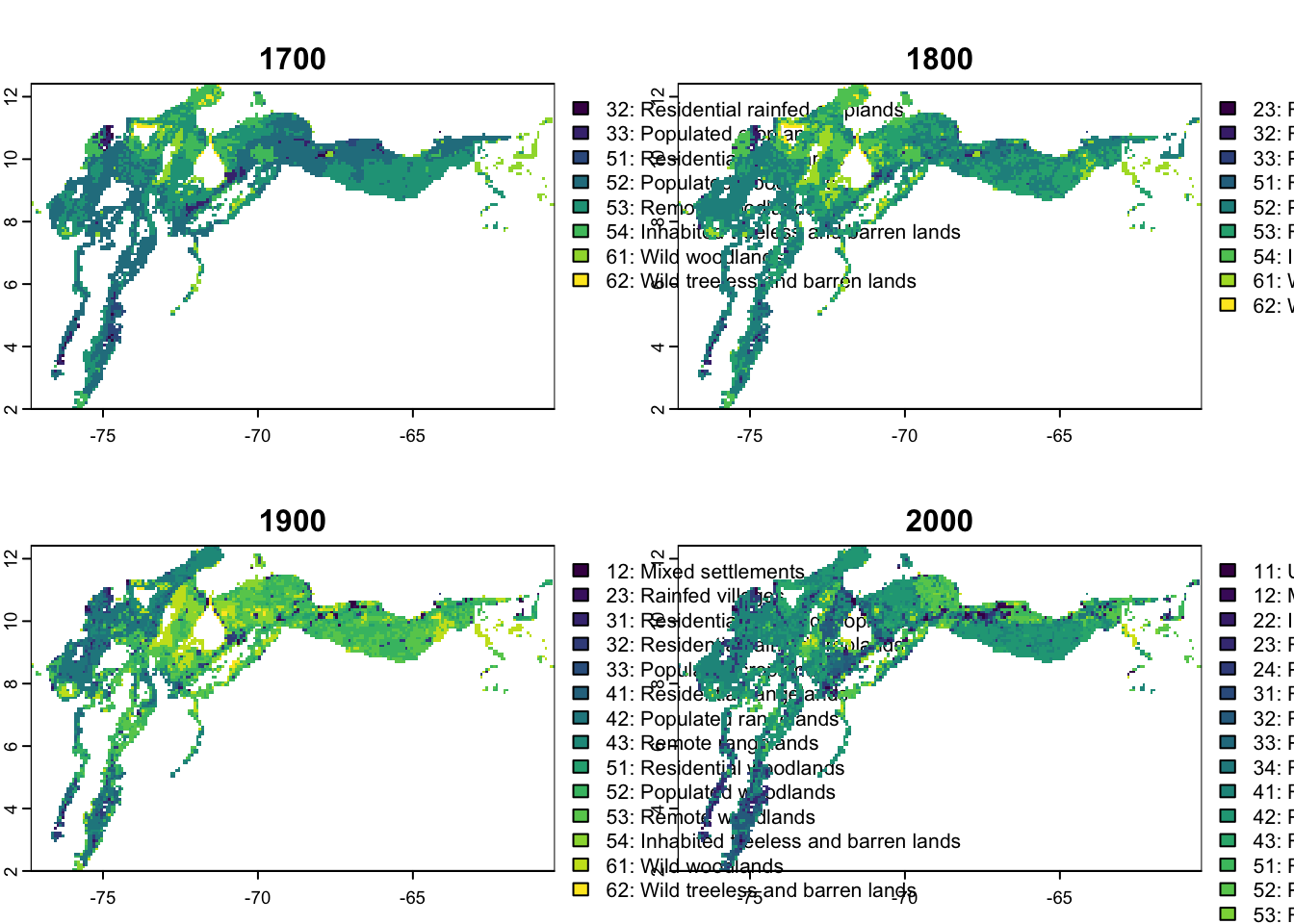

For the next step we need to now the values of the categories of interest. Here we filter the categories with “woodlands” in their label:

(slc_cats <- cats(anthromes)[[2]] |> 
  filter(grepl("woodlands", LABEL)))

  VALUE                     LABEL
1    51 51: Residential woodlands
2    52   52: Populated woodlands
3    53      53: Remote woodlands
4    61        61: Wild woodlands

10.3 Data preparation

Calculate areas from maps

We calculate the sum of the areas of all cells in the four categories associated with “woodlands” in the Anthromes dataset. We apply this calculation to all four maps representing four epochs from 1700 to 2000:

cell_areas <- values(cellSize(anthromes, unit = 'km'))
cell_selection <- values(anthromes %in% slc_cats$VALUE)

y <- apply(cell_selection, 2, function(x) {sum(x*cell_areas)})
x <- seq(1700,2000, by = 100)
tibble(year = x, `woodland area estimate` = y)

# A tibble: 4 × 2
   year `woodland area estimate`
  <dbl>                    <dbl>
1  1700                  366850.
2  1800                  368110.
3  1900                  262671.
4  2000                   71025.

This plot allow us to visualise the four estimates. The values at 1700 and 1800 are very similar, with a pronounced decline afterwards. This suggests that the declines in woodland areas were not linear during these 300 years.

baseplot <- 
    ggplot() +
    geom_point(aes(x = x, y = y), colour = 'black', cex = 2) +
    labs(y = "Estimated woodland area [km^2]", x = "Year") +
    theme_bw()

baseplot +
  labs(title = "Four point estimates of woodland area")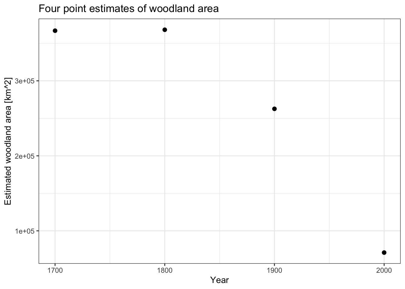

Decline statistics

Rate of change

The function getDeclineStats from the redlistr package offers three methods to estimate the rate of decline from two point estimates of area (Lee and Murray 2023). Since we expect small changes prior to 1800, we can use the year 1800 and the year 2000 to estimate the historical rate of decline using different formulas:

DS_hist <- getDeclineStats(y[2], y[4], year.t1 = x[2], year.t2 = x[4],
                                 methods = c('PRD', 'ARD', 'ARC'))

DS_hist

     absolute.loss      ARD       PRD       ARC
1800      297084.9 1485.424 0.8193022 -0.822677

And the same for the period between 1900 and 2000

DS_pres <- getDeclineStats(y[3], y[4], year.t1 = x[3], year.t2 = x[4],
                                 methods = c('PRD', 'ARD', 'ARC'))

DS_pres

     absolute.loss      ARD      PRD       ARC
1900      191646.8 1916.468 1.299362 -1.307877

GLM approach

In José Rafael Ferrer-Paris et al. (2019) a quasipoisson GLM with log-link function was used for interpolation of changes in the dependant variable (Woodland area) because it provides a convenient function to calculate variable proportional rates of decline. In this case we use a polynomial term to account for non-linear relationships between the four point estimates. In this case the GLM function is used for convenience, not as a statistical model for inference, but only as a function for interpolation.

glm02 <-  glm(y~poly(x,2), family = quasipoisson(log))
summary(glm02)

Call:
glm(formula = y ~ poly(x, 2), family = quasipoisson(log))

Coefficients:
            Estimate Std. Error t value Pr(>|t|)   
(Intercept) 12.33296    0.08474 145.532  0.00437 **
poly(x, 2)1 -1.12424    0.18948  -5.933  0.10630   
poly(x, 2)2 -0.59467    0.15920  -3.735  0.16652   
---
Signif. codes:  0 '***' 0.001 '**' 0.01 '*' 0.05 '.' 0.1 ' ' 1

(Dispersion parameter for quasipoisson family taken to be 5261.672)

    Null deviance: 271520.5  on 3  degrees of freedom
Residual deviance:   5239.9  on 1  degrees of freedom
AIC: NA

Number of Fisher Scoring iterations: 4

Extrapolation

Rate of change

Using the rate of of change approach, we now need to extrapolate the expected area for the year of interest. We use function extrapolateEstimate from redlistr.

y_hist <- foreach(nY=c(200,225), .combine = "bind_rows")  %do% {
    extrapolateEstimate(y[2],  year.t1 = x[2], nYears = nY,
                                  PRD = DS_hist$PRD,
                                  ARD = DS_hist$ARD,
                                  ARC = DS_hist$ARC)
}
y_hist

         forecast.year A.ARD.t3 A.PRD.t3 A.ARC.t3
1800...1          2000 71024.62 71024.62 71024.62
1800...2          2025 33889.01 57821.30 57821.30

And we can do the same for the more recent estimates of rates of decline and shorter time frames:

y_pres <- foreach(nY=c(50,75,100,125), .combine = "bind_rows")  %do% {
    extrapolateEstimate(y[3],  year.t1 = x[3], nYears = nY,
                                  PRD = DS_pres$PRD,
                                  ARD = DS_pres$ARD,
                                  ARC = DS_pres$ARC)
}
y_pres

         forecast.year  A.ARD.t3  A.PRD.t3  A.ARC.t3
1900...1          1950 166848.03 136587.48 136587.48
1900...2          1975 118936.32  98494.03  98494.03
1900...3          2000  71024.62  71024.62  71024.62
1900...4          2025  23112.91  51216.27  51216.27

Notice that the forecasts of area for the year 2000 will be the same as the estimated area straight from the map calculations. For extrapolation to 2025, the forecast based on absolute rate of decline (ARD) is lower than the one for proportional rate of decline (PRD). In this example, the proportional rate of decline is the preferred approach as it seems to be a more realistic scenario of future changes.

GLM approach

For the GLM approach we use the predict function to get the expected and standard error values in the scale of the response:

nwdt <- data.frame(x=seq(1700,2000,25))

prd01 <- predict(
    glm02,
    newdata = nwdt,
    type = "response",
    se.fit = T)

nwdt$y <- prd01$fit
nwdt$y_se <-  prd01$se.fit 

And we use the prediction in the log scale to construct a plausible interval using the standard error and a normal distribution approximation for 90% intervals.

prd02 <- predict(
    glm02,
    newdata = nwdt,
    type = "link",
    se.fit = T)
nwdt$upper <- exp(prd02$fit + (1.645*prd02$se.fit))
nwdt$lower <- exp(prd02$fit - (1.645*prd02$se.fit))

The use of the GLM allows a continuous prediction of the expected values and plausible intervals as shown in the plot:

(predplot <- baseplot +
    geom_ribbon(
      data = nwdt, 
      aes(x = x,ymin = lower,ymax = upper), 
      fill = 'grey', alpha = .5) +
    geom_line(
      data = nwdt, 
      aes(x = x, y = y), 
      colour = 'black', lwd = 1.2, alpha = .5) ) +
    labs(
      title = "Interpolated estimates of woodland area per year",
      subtitle = "Including uncertainty in the interpolation")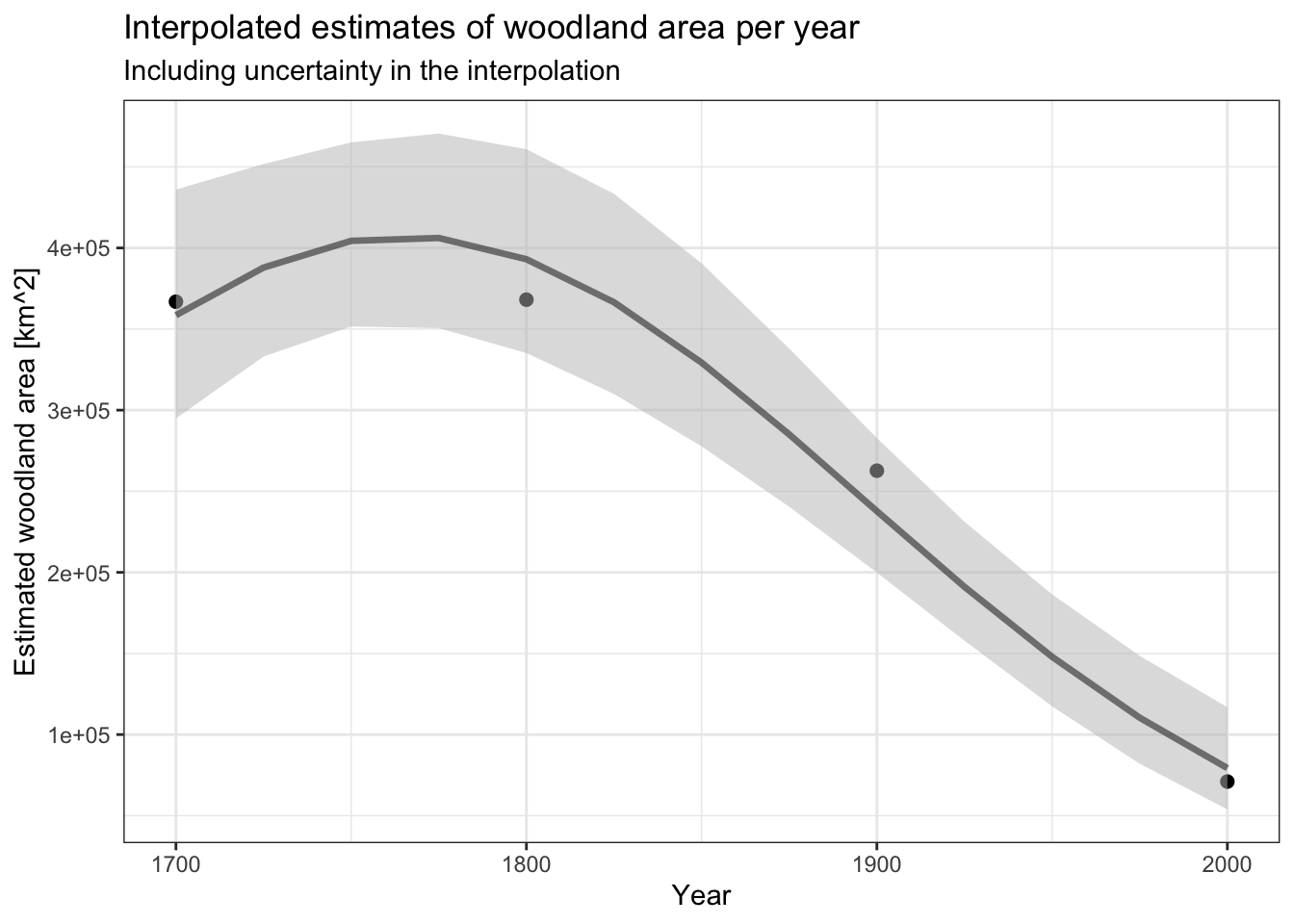

10.4 Assessment of subcriteria

For this two subcriteria will use this function implemented by José R. Ferrer-Paris et al. (2024) to calculate the percentage of decline in area based on intial (start) and final values (end). The function uses an error propagation formula to estimate the error of the output estimate based on the errors of the input estimates (if known).

calc_decline <- function(data,start,end) {
  stopifnot("eco_extent" %in% colnames(data),
            "years" %in% colnames(data),
            start<=nrow(data),
            end<=nrow(data))
  start_date <- pull(data[start,"years"])
  end_date <- pull(data[end,"years"])
  stopifnot(start_date<end_date)
  start_extent <- pull(data[start,"eco_extent"])
  end_extent <- pull(data[end,"eco_extent"])
  res <- dplyr::tibble(
    start_date,
    end_date,
    time_frame = end_date-start_date,
    decline = (units::set_units(1,'1') - 
                 (end_extent/start_extent)) %>% 
      units::set_units('%')
      )
  if ("error_extent" %in% colnames(data)) {
    start_error <- pull(data[start,"error_extent"])
    end_error <- pull(data[end,"error_extent"])
    res$error <- sqrt(((end_extent^2 * start_error^2) + (start_extent^2 * end_error^2)) / (start_extent^4)) %>% units::set_units('%')
  }
  return(res)
}

Subcriterion A1

The estimated percentage of decline between years 1950 and 2000 and between 1975 and 2025 will be the same when using a proportional rate of decline because the rate is linear in the log-scale and the time period is the same:

y_pres <- tibble(y_pres) |> 
  transmute(
    eco_extent=set_units(A.PRD.t3,'km2'), 
    years=forecast.year) 

calc_decline(y_pres, start=2, end=4)

# A tibble: 1 × 4
  start_date end_date time_frame decline
       <dbl>    <dbl>      <dbl>     [%]
1       1975     2025         50    48.0

calc_decline(y_pres, start=1, end=3)

# A tibble: 1 × 4
  start_date end_date time_frame decline
       <dbl>    <dbl>      <dbl>     [%]
1       1950     2000         50    48.0

The point estimates based on two measurements do not include a measure of uncertainty.

The estimated percentage decline using the GLM predictions from 1950 and 2000 are close to the estimates from the rates of decline, but the error is relatively large, meaning that there is considerable uncertainty in the extrapolation:

y_glm <- tibble(nwdt) |> 
  filter(x %in% c(1950,2000)) |> 
  transmute(
    years = x,
    eco_extent = set_units(y,'km2'),
    error_extent = set_units(y_se,'km2')
  )

calc_decline(y_glm, start=1, end=2)

# A tibble: 1 × 5
  start_date end_date time_frame decline error
       <dbl>    <dbl>      <dbl>     [%]   [%]
1       1950     2000         50    46.4  14.7

This uncertainty is reflected in the plot, and when combined with the RLE thresholds for this criterion suggest a plausible range of categories between LC and EN.

barx <- c(2005,2015)
thrs <- c(0,.2,.5,.7,1)
clrs <- c("red","orange","yellow","darkgreen")
IV <- nwdt |> filter(x %in% c(1950)) |> pull(y)

predplot +
annotate("rect", 
  xmin = barx[1],
  xmax = barx[2],
  ymin = IV*thrs[-5],
  ymax = IV*thrs[-1], 
  fill = clrs,  alpha = .7) +
scale_y_continuous(
    name = "Estimated woodland area [km^2]",
    sec.axis = sec_axis(~.*100/IV, name="Remaining woodland cover [%]",
    breaks=thrs * 100)
  ) +
  labs(title="Subcriterion A1", subtitle = "Baseline 1950")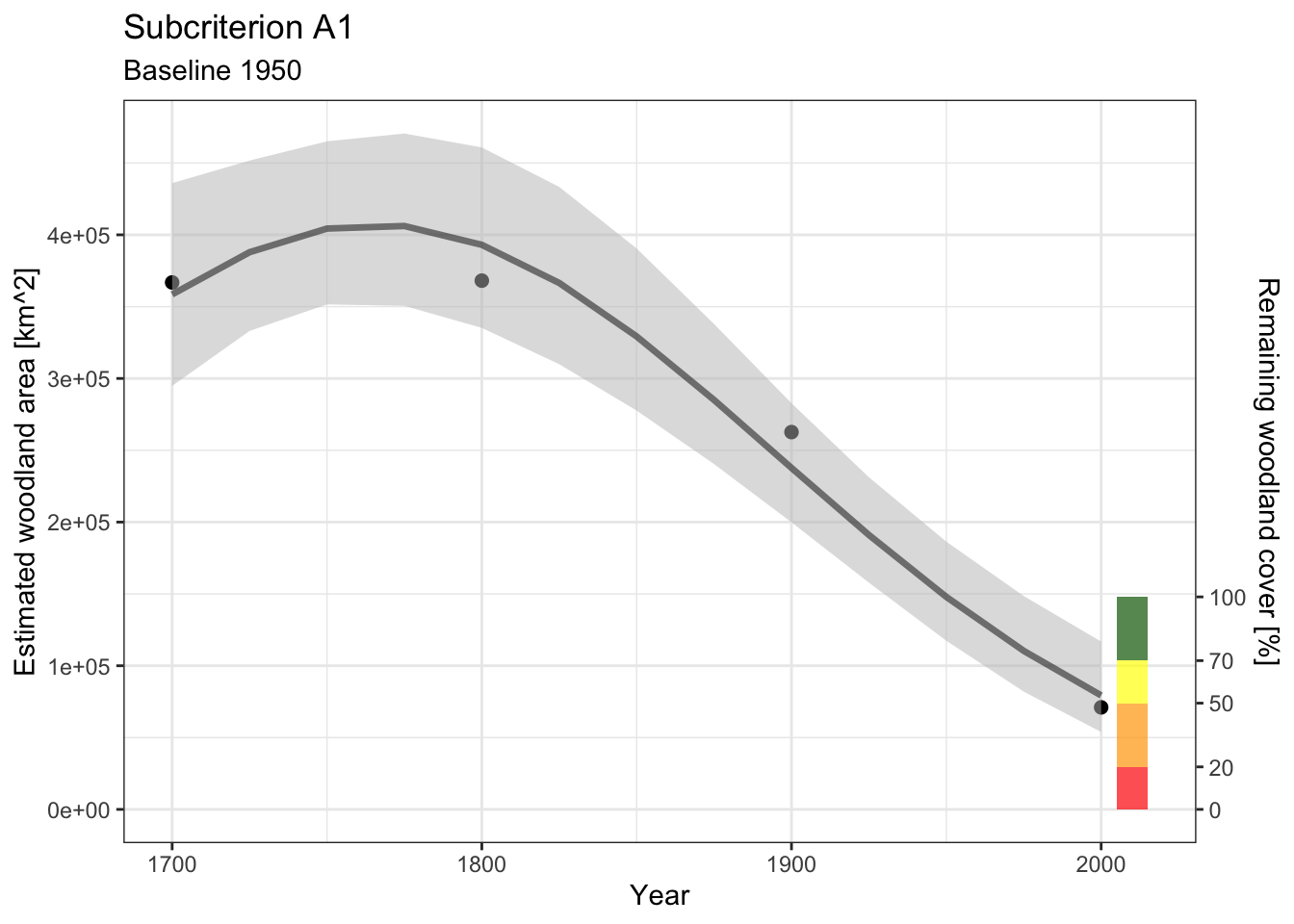

Subcriterion A3

For subcriterion A3 we need to combine the estimates based on the map calculations (1700 to 2000) with the extrapolated values for the present day (2025):

y_hist <-  tibble(
    years = x, eco_extent= set_units(y,'km2')) |> 
  bind_rows(
  {
  tibble(y_hist) |> 
    transmute(
      eco_extent=set_units(A.PRD.t3,'km2'), 
      years=forecast.year) 
  }
)
y_hist

# A tibble: 6 × 2
  years eco_extent
  <dbl>     [km^2]
1  1700    366850.
2  1800    368110.
3  1900    262671.
4  2000     71025.
5  2000     71025.
6  2025     57821.

calc_decline(y_hist, start=1, end=4)

# A tibble: 1 × 4
  start_date end_date time_frame decline
       <dbl>    <dbl>      <dbl>     [%]
1       1700     2000        300    80.6

calc_decline(y_hist, start=1, end=6)

# A tibble: 1 × 4
  start_date end_date time_frame decline
       <dbl>    <dbl>      <dbl>     [%]
1       1700     2025        325    84.2

The point estimates are between 80 and 85 %.

Using the function with the GLM data between 1750 and 2000 we get:

y_glm <- tibble(nwdt) |> 
  filter(x %in% c(1750,2000)) |> 
  transmute(
    years = x,
    eco_extent = set_units(y,'km2'),
    error_extent = set_units(y_se,'km2')
  )

calc_decline(y_glm, start=1, end=2)

# A tibble: 1 × 5
  start_date end_date time_frame decline error
       <dbl>    <dbl>      <dbl>     [%]   [%]
1       1750     2000        250    80.4  4.91

For this case the estimated error is relatively small, and suggests that the estimated decline is well above 70% (threshold for EN) but still below 90% (threshold for CR).

thrs <- c(0,.1,.3,.5,1)
IV <- nwdt |> filter(x %in% c(1750)) |> pull(y)

predplot +
annotate("rect", 
  xmin = barx[1],
  xmax = barx[2],
  ymin = IV*thrs[-5],
  ymax = IV*thrs[-1], 
  fill = clrs,  alpha = .7) +
scale_y_continuous(
    name = "Estimated woodland area [km^2]",
    sec.axis = sec_axis(~.*100/IV, name="Remaining woodland cover [%], baseline 1750",
    breaks = thrs * 100)
  ) +
  labs(title="Subcriterion A3")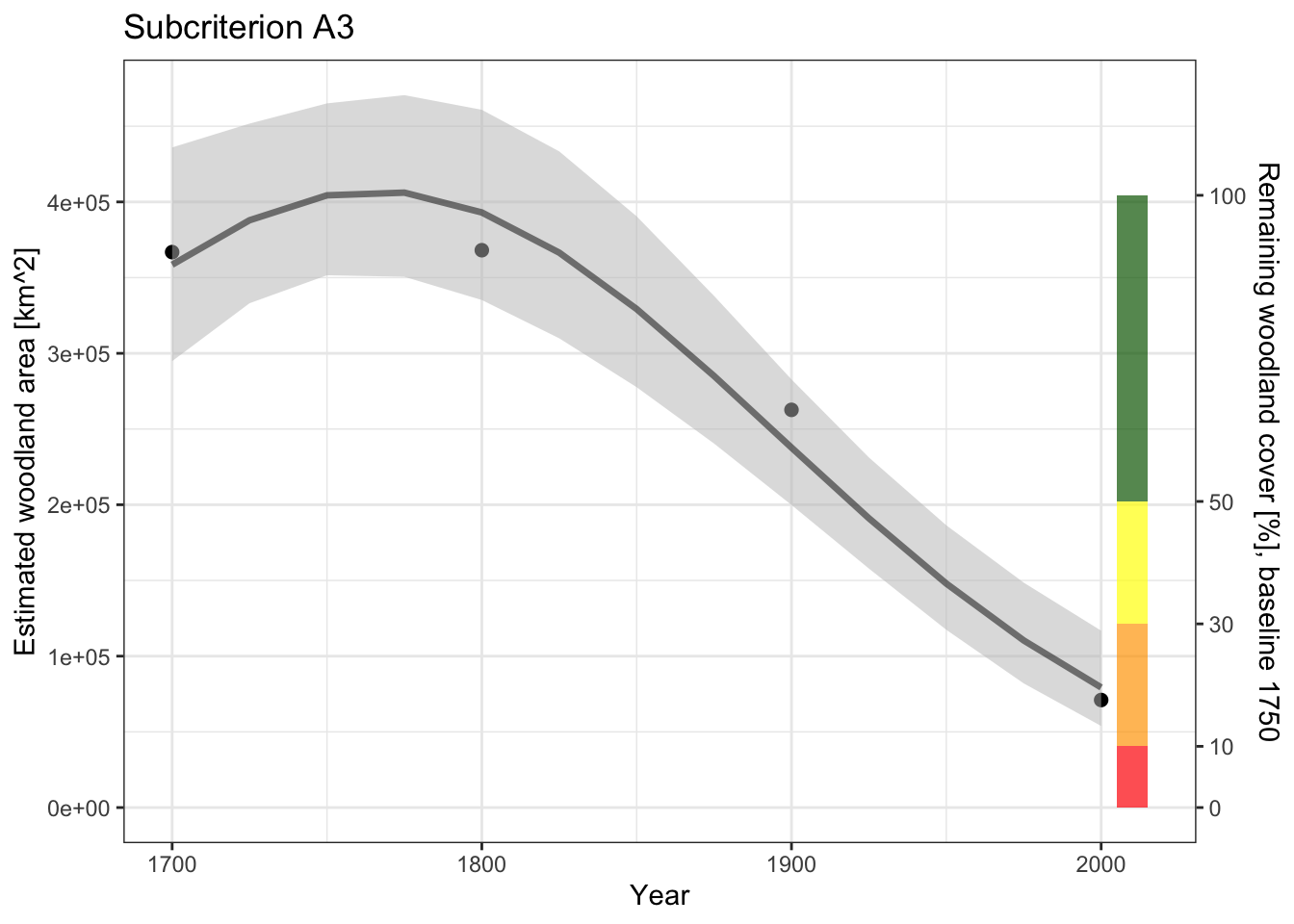

The visualisation also suggests that the most plausible category is EN.

Ellis, Erle C. 2019. “Anthromes_2_GeoTIFF.zip.” In Anthromes V2 (GeoTiff). Harvard Dataverse. https://doi.org/10.7910/DVN/6KKAWS/95LDTT.

Ferrer-Paris, José Rafael, Irene Zager, David A. Keith, María A. Oliveira-Miranda, Jon Paul Rodríguez, Carmen Josse, Mario González-Gil, Rebecca M. Miller, Carlos Zambrana-Torrelio, and Edmund Barrow. 2019. “An Ecosystem Risk Assessment of Temperate and Tropical Forests of the Americas with an Outlook on Future Conservation Strategies.” Conservation Letters 12 (2): e12623. https://doi.org/10.1111/conl.12623.

Ferrer-Paris, José R., Luis Daniel Llambí, Alejandra Melfo, and David Keith. 2024. “First Red List of Ecosystems Assessment of a Tropical Glacier Ecosystem to Diagnose the Pathways Toward Imminent Collapse.” Oryx Published online: 1–11. https://doi.org/10.1017/S0030605323001771.

Lee, Calvin, and Nicholas Murray. 2023. Redlistr: Tools for the IUCN Red List of Ecosystems and Species. https://doi.org/10.32614/CRAN.package.redlistr.