12  Subcriterion A2b

Reproducible workflow using Python

This document shows an example calculation of criterion B using data assets and functions available on Earth Engine (EE) from a notebook running Python.

12.1 Updating the assessment workflow

The original workflow included a combination of two remote sensing products (Friedl et al. 2010; Hansen et al. 2013). The updated workflow is based on an updated version of one data source that spans more years and uses improved algorithms. We have two version of the workflow, one based on R and local copies of the remote sensing products (see Section 11.1), and one based on Python and Earth Engine for cloud computing (this document).

Differences between original and updated assessment workflows for subcriterion A2b.

Step	2019	2025 (R)	2025 (Python)
GIS data prep.	GRASS GIS / gdal / R	R / gdal / terra	Earth Engine
Data source	GFC v1.2 (2015) and MODIS LC v5.1	GFC v1.12 (2024)	GFC v1.12 (2024)
Analysis	R / glm	R / glm / redlistr	Python / Earth Engine
Timeframe	2000-2050	2000-2050	2000-2050

Part of the code is based on examples from Earth Engine Guides.

12.2 Set up

Import modules

import ee
import geemap.core as geemap
import pandas as pd
import pyreadr

import numpy as np
import statsmodels.api as sm
import matplotlib.pyplot as plt

Authenticate to Earth Engine

myproject='ee-jrferrerparis'

ee.Authenticate()
ee.Initialize(project=myproject)

Read inputs

Here we will use three assets, two of them are available in Earth Engine’s data catalog:

gfc=ee.Image('UMD/hansen/global_forest_change_2024_v1_12')
countries=ee.FeatureCollection('USDOS/LSIB_SIMPLE/2017')

The third asset has been uploaded from (FerrerParis20025?) into my personal project:

macrogroups=ee.Image('projects/{}/assets/IVC_NS_v7_270m_cea'.format(myproject))

12.3 Prepare the data

First we need to select the target macrogroup, in this case the raster value is the ID, so value 563 returns the potential distribution of M563:

MG563 = macrogroups.eq(563);

Then we define a region of interest, in this case we know this macrogroup is present in three countries: Colombia, Venezuela, and Trinidad and Tobago, so we will create regions for each one of them.

rVEN = countries.filter(
    ee.Filter.inList('country_na', ['Venezuela',])
)
rCOL = countries.filter(
    ee.Filter.inList('country_na', ['Colombia',])
)
rTT = countries.filter(
    ee.Filter.inList('country_na', ['Trinidad & Tobago',])
)

Parameters and functions

We set up the scale for the outputs

params = {'scale': 30, 'maxPixels':1e10}

And calculate the corresponding resolution

res_km2 = (params['scale']**2)/1e6

Now we design our own combined reducer for the spatial analysis:

combinedReducer = ee.Reducer.sum().combine(
  reducer2 = ee.Reducer.count(),
  sharedInputs = True 
).combine(
  reducer2 = ee.Reducer.mean(),
  sharedInputs = True 
)

12.4 Analysis approach: Compute totals

The first approach is to calculate raster totals and do the calculations afterwards. We choose treecover, gain and loss bands from GFC and apply the mask for the potential distribution of our target macrogroup.

mcdgTotals = (
    gfc
    .select(['treecover2000','gain','loss'])
    .selfMask()
    .mask(MG563)
)

Computations

We compute summaries of the three bands for each country

totalsVEN = mcdgTotals.reduceRegion(
    reducer=combinedReducer,
    geometry=rVEN.geometry(),
    scale=params['scale'],
    maxPixels=params['maxPixels'],
).getInfo()

totalsVEN

{'gain_count': 105206342,
 'gain_mean': 0.0040003273355281,
 'gain_sum': 420784.8392156863,
 'loss_count': 105206342,
 'loss_mean': 0.0586245309569536,
 'loss_sum': 6166573.823529413,
 'treecover2000_count': 105206342,
 'treecover2000_mean': 37.97777763966412,
 'treecover2000_sum': 3994791355.184314}

totalsCOL = mcdgTotals.reduceRegion(
    reducer=combinedReducer,
    geometry=rCOL.geometry(),
    scale=params['scale'],
    maxPixels=params['maxPixels'],
).getInfo()

totalsTT = mcdgTotals.reduceRegion(
    reducer=combinedReducer,
    geometry=rTT.geometry(),
    scale=params['scale'],
    maxPixels=params['maxPixels'],
).getInfo()

Aggregate results

totals = pd.DataFrame([totalsVEN,totalsCOL,totalsTT])

totals

	gain_count	gain_mean	gain_sum	loss_count	loss_mean	loss_sum	treecover2000_count	treecover2000_mean	treecover2000_sum
0	105206342	0.004000	420784.839216	105206342	0.058625	6.166574e+06	105206342	37.977778	3.994791e+09
1	54502069	0.014495	789892.454902	54502069	0.103135	5.620141e+06	54502069	35.044587	1.909694e+09
2	233854	0.003176	741.000000	233854	0.045033	1.050737e+04	233854	75.694211	1.766134e+07

totals['eco_extent_2000'] = (totals.treecover2000_sum / 100) * res_km2 

totals['eco_extent_2024'] = totals['eco_extent_2000'] - ((totals.loss_sum.sum()) * res_km2) + ((totals.gain_sum.sum()) * res_km2)

totals[['eco_extent_2000','eco_extent_2024']]

	eco_extent_2000	eco_extent_2024
0	35953.122197	26425.898653
1	17187.244420	7660.020876
2	158.952065	-9368.271479

12.5 Analysis approach: Raster algebra

The second approach is to use raster algebra to calculate a new image of tree cover for 2024 that reflects pixel by pixel changes.

mcdg_2024 = (
    gfc
    .select(['treecover2000'])
    .multiply(gfc.select(['loss']).eq(0))
    .add(gfc.select(['gain']).multiply(100))
    .mask(MG563)
)

Computations

finalVEN = mcdg_2024.reduceRegion(
    reducer=combinedReducer,
    geometry=rVEN.geometry(),
    scale=params['scale'],
    maxPixels=params['maxPixels'],
).getInfo()

finalCOL = mcdg_2024.reduceRegion(
    reducer=combinedReducer,
    geometry=rCOL.geometry(),
    scale=params['scale'],
    maxPixels=params['maxPixels'],
).getInfo()

finalTT = mcdg_2024.reduceRegion(
    reducer=combinedReducer,
    geometry=rTT.geometry(),
    scale=params['scale'],
    maxPixels=params['maxPixels'],
).getInfo()

Aggregate results

finals = pd.DataFrame([finalVEN,finalCOL,finalTT])

finals

	treecover2000_count	treecover2000_mean	treecover2000_sum
0	105206342	34.141011	3.591211e+09
1	54502069	28.821156	1.570559e+09
2	233854	71.958293	1.678966e+07

finals['treecover2000_sum'] / totals['treecover2000_sum'] 

0    0.898973
1    0.822414
2    0.950645
Name: treecover2000_sum, dtype: float64

sum(finals['treecover2000_sum']) / sum(totals['treecover2000_sum'] )

0.8744396077079528

253656.4 / sum(totals['gain_count'])

0.0015859247710416004

12.6 Analysis approach: Cross tabulation

A third approach is to do a crosstabulation of tree cover loss per year, we use the bands treecover2000 and lossyear from the GFC dataset.

mcdgTC = (
    gfc
    .select(['treecover2000','lossyear'])
    .mask(MG563)
)

Computations

tclVEN = mcdgTC.reduceRegion(
    reducer=combinedReducer.group(groupField=1, groupName='lossyear'),
    geometry=rVEN.geometry(),
    scale=params['scale'],
    maxPixels=params['maxPixels'],
).getInfo()

tclCOL = mcdgTC.reduceRegion(
    reducer=combinedReducer.group(groupField=1, groupName='lossyear'),
    geometry=rCOL.geometry(),
    scale=params['scale'],
    maxPixels=params['maxPixels'],
).getInfo()

tclTT = mcdgTC.reduceRegion(
    reducer=combinedReducer.group(groupField=1, groupName='lossyear'),
    geometry=rTT.geometry(),
    scale=params['scale'],
    maxPixels=params['maxPixels'],
).getInfo()

Crosstabulation of loss per year

Create a function to prepare the results of the previous computation for the extrapolation step:

def prepareDF(r1,r2):
    # We read the data from the treecover / lossyear crosstabulation:
    df = pd.DataFrame(r1['groups'])
    # We use the values calculated from the gain layer to correct the area estimates:
    df['gain'] = (r2['gain_sum'] / 24)
    df.loc[df.lossyear==0,'gain'] = 0
    # We calculate the area for each year by dividing the treecover by 100, 
    # adding a portion of the gain and using the resolution to transform to area:
    df['tc_area'] = df['area'] = ((df['sum']/100) + df['gain']) * res_km2 
    # We reorder the data to account for the area lost between 2001 and 2024 and the area remaining in 2025
    df['order'] = 25 - df['lossyear']
    df['year'] = 1999 + df['lossyear']
    df.loc[df.lossyear==0,'order'] = 0
    df.loc[df.lossyear==0,'year'] = 2025
    df.sort_values('order', inplace=True)
    # Now calculate the accumulated area in reverse order of years:
    df['tc_area'] = np.cumsum( df['area'])
    # And reorder to get a time series of remaining area per year:
    df.sort_values('year', inplace=True)
    return(df)

Apply this function to the data from Venezuela

resultsVEN = prepareDF(tclVEN,totalsVEN)

resultsVEN.head()

	count	lossyear	mean	sum	gain	tc_area	area	order	year
1	352765	1	73.815910	2.603826e+07	17532.701634	36331.828552	250.123728	24	2000
2	224563	2	74.279556	1.667921e+07	17532.701634	36081.704824	165.892364	23	2001
3	217493	3	80.186956	1.743915e+07	17532.701634	35915.812460	172.731799	22	2002
4	188625	4	74.362437	1.402577e+07	17532.701634	35743.080661	142.011373	21	2003
5	241077	5	75.143395	1.811477e+07	17532.701634	35601.069287	178.812379	20	2004

Apply this function to the data from Colombia

resultsCOL = prepareDF(tclCOL,totalsCOL)

Apply this function to the data from Trinidad and Tobago

resultsTT = prepareDF(tclTT,totalsTT)

12.7 Extrapolation of decline

Xnew=pd.DataFrame(range(2000,2050),columns=['year',]).assign(intercept=1)
Xnew['year_squared'] = Xnew['year']**2

def fitExtModel(df):
    X = (df
         .assign(intercept=1)
         .reset_index(drop=True)
        )
    X['year_squared'] = X['year']**2
    y = X.pop('tc_area')
    model_1 = sm.GLM(
        y,
        X[['intercept', 'year', 'year_squared']],
        family=sm.families.Poisson(),
        )
    return model_1.fit()

extVEN = fitExtModel(resultsVEN)
print(extVEN.summary())

                 Generalized Linear Model Regression Results                  
==============================================================================
Dep. Variable:                tc_area   No. Observations:                   25
Model:                            GLM   Df Residuals:                       22
Model Family:                 Poisson   Df Model:                            2
Link Function:                    Log   Scale:                          1.0000
Method:                          IRLS   Log-Likelihood:                -159.71
Date:                Mon, 25 Aug 2025   Deviance:                       12.561
Time:                        20:38:29   Pearson chi2:                     12.6
No. Iterations:                     3   Pseudo R-squ. (CS):              1.000
Covariance Type:            nonrobust                                         
================================================================================
                   coef    std err          z      P>|z|      [0.025      0.975]
--------------------------------------------------------------------------------
intercept      -98.7564     90.558     -1.091      0.275    -276.247      78.735
year             0.1140      0.090      1.266      0.205      -0.062       0.290
year_squared -2.968e-05   2.24e-05     -1.327      0.185   -7.35e-05    1.42e-05
================================================================================

prdVEN=extVEN.get_prediction(Xnew[['intercept', 'year', 'year_squared']]).summary_frame()

plt.plot(resultsVEN[['year']], resultsVEN[['tc_area']], 'o')
plt.plot(Xnew[['year']], prdVEN["mean"], '--', label='fit')
plt.ylabel("Area estimated from tree cover %")
plt.xlabel("Year")
plt.fill_between(
    Xnew['year'], prdVEN["mean_ci_lower"], prdVEN["mean_ci_upper"], color="k", alpha=0.1,
    label='plausible range'
);
plt.legend()
plt.show()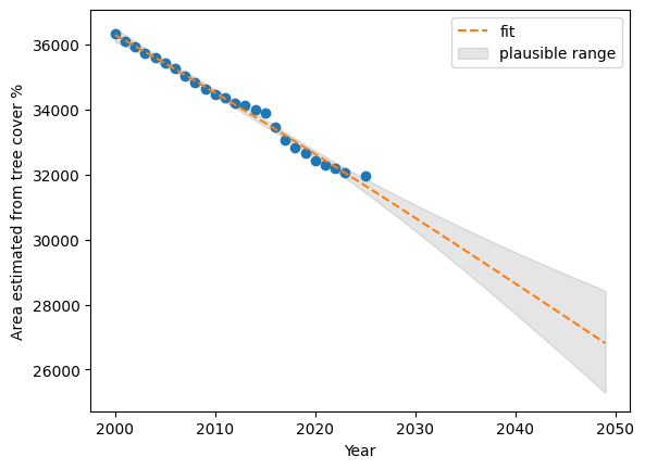

100 - (prdVEN.iloc[49][["mean","mean_ci_lower","mean_ci_upper"]].values * 100 / resultsVEN.iloc[0][['tc_area']].values)

array([26.20915397, 30.41213941, 21.75231554])

extCOL = fitExtModel(resultsCOL)
prdCOL=extCOL.get_prediction(Xnew[['intercept', 'year', 'year_squared']]).summary_frame()
100 - (prdCOL.iloc[49][["mean","mean_ci_lower","mean_ci_upper"]].values * 100 / resultsCOL.iloc[0][['tc_area']].values)

array([52.71523956, 56.68077749, 48.38668748])

plt.plot(resultsCOL[['year']], resultsCOL[['tc_area']], 'o')
plt.plot(Xnew[['year']], prdCOL["mean"], '--', label='fit')
plt.ylabel("Area estimated from tree cover %")
plt.xlabel("Year")
plt.fill_between(
    Xnew['year'], prdCOL["mean_ci_lower"], prdCOL["mean_ci_upper"], color="k", alpha=0.1,
    label='plausible range'
);
plt.legend()
plt.show()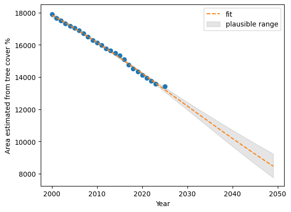

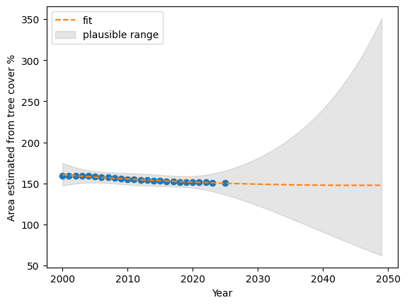
extTT = fitExtModel(resultsTT)
prdTT=extTT.get_prediction(Xnew[['intercept', 'year', 'year_squared']]).summary_frame()
prdTT.iloc[49][["mean","mean_ci_lower","mean_ci_upper"]].values * 100 / resultsTT.iloc[0][['tc_area']].values

array([ 92.5565775 ,  38.95877469, 219.89192697])

resultsTT.iloc[0][['tc_area']].values

array([159.61896455])

plt.plot(resultsTT[['year']], resultsTT[['tc_area']], 'o')
plt.plot(Xnew[['year']], prdTT["mean"], '--', label='fit')
plt.ylabel("Area estimated from tree cover %")
plt.xlabel("Year")
plt.fill_between(
    Xnew['year'], prdTT["mean_ci_lower"], prdTT["mean_ci_upper"], color="k", alpha=0.1,
    label='plausible range'
);
plt.legend()
plt.show()

Friedl, Mark A., Damien Sulla-Menashe, Bin Tan, Annemarie Schneider, Navin Ramankutty, Adam Sibley, and Xiaoman Huang. 2010. “MODIS Collection 5 Global Land Cover: Algorithm Refinements and Characterization of New Datasets.” Remote Sensing of Environment 114 (1): 168–82. https://doi.org/https://doi.org/10.1016/j.rse.2009.08.016.

Hansen, M. C., P. V. Potapov, R. Moore, M. Hancher, S. A. Turubanova, A. Tyukavina, D. Thau, et al. 2013. “High-Resolution Global Maps of 21st-Century Forest Cover Change.” Science 342 (6160): 850–53. https://doi.org/10.1126/science.1244693.