from pyinaturalist import get_observations
import geopandas as gpd
import pandas as pd
import numpy as np
from shapely.geometry import Point
from mpl_toolkits.basemap import Basemap
import matplotlib.pyplot as plt
import plotly.express as px
import zipfile, requests, io
import pyprojrootAround the world with iNaturalist
Python
Plotly
Geopandas
global
basemap
Mapping Biodiversity: Visualizing iNaturalist Observations with Python
Today, we’ll embark on an adventure from the field to the digital realm. Let’s explore how to extract, map, and analyze global iNaturalist observations using Python.
Overview
In this blog post, we’ll walk through the following steps to map and analyze iNaturalist observations using Python:
- Download iNaturalist observations from around the world.
- Display these observations on a world map.
- Intersect observations with country and national boundaries.
- Generate interactive graphs to explore observations at different levels.
Tools and Libraries
I will be using a Python environment with a selection of my favourite libraries, as explained here.
We will be using the following libraries in this blog post:
pyinaturalist: A Python client for the iNaturalist API, allowing access to observation data.
Matplotlib basemap toolkit: A library for plotting 2D data on maps in Python.
geopandas: An extension of pandas that supports spatial data operations, making it easier to work with geographic datasets.
plotly: A graphing library that makes interactive plots and dashboards with ease.
Declare the root folder for the repository:
repodir = pyprojroot.find_root(pyprojroot.has_dir(".git"))Step-by-Step Guide
Step 1: Downloading iNaturalist Observations
Let’s begin by fetching iNaturalist observations with pyinaturalist. We will need a selection of global observations so we select the user neomapas1, and see where in the world they have been.
username = 'neomapas'
observations = get_observations(user_id=username, per_page=0)
n_obs = observations['total_results']

# First we need to figure out how many observations to expect:
print("User _{}_ has {} observations in iNaturalist".format(username,n_obs))
User _neomapas_ has 3324 observations in iNaturalistThe maximum number of observations we can download in each query 200, so we need to use pagination to get all results. For each query we will extract a minimum selection of fields that we will use for summarising the data (coordinates, place and species guess), but there are many other fields that could be important to include for more in depth explorations.
records=list()
j=1
while len(records) < n_obs:
    print("Requesting observations from user _{}_: page {}, total of {} observations downloaded".format(username,j,min(j*200,n_obs)))
    observations = get_observations(user_id=username,per_page=200,page=j)
    for obs in observations['results']:
        record = {
            'longitude': obs['location'][1],
            'latitude': obs['location'][0],
            'location': obs['place_guess'],
            'species guess': obs['species_guess'],
        }
        if len(obs['observation_photos'])>0:
            record['url'] = obs['observation_photos'][0]['photo']['url']
            record['attribution'] = obs['observation_photos'][0]['photo']['attribution']
        records.append(record)
    j=j+1
Requesting observations from user _neomapas_: page 1, total of 200 observations downloaded
Requesting observations from user _neomapas_: page 2, total of 400 observations downloaded
Requesting observations from user _neomapas_: page 3, total of 600 observations downloaded
Requesting observations from user _neomapas_: page 4, total of 800 observations downloaded
Requesting observations from user _neomapas_: page 5, total of 1000 observations downloaded
Requesting observations from user _neomapas_: page 6, total of 1200 observations downloaded
Requesting observations from user _neomapas_: page 7, total of 1400 observations downloaded
Requesting observations from user _neomapas_: page 8, total of 1600 observations downloaded
Requesting observations from user _neomapas_: page 9, total of 1800 observations downloaded
Requesting observations from user _neomapas_: page 10, total of 2000 observations downloaded
Requesting observations from user _neomapas_: page 11, total of 2200 observations downloaded
Requesting observations from user _neomapas_: page 12, total of 2400 observations downloaded
Requesting observations from user _neomapas_: page 13, total of 2600 observations downloaded
Requesting observations from user _neomapas_: page 14, total of 2800 observations downloaded
Requesting observations from user _neomapas_: page 15, total of 3000 observations downloaded
Requesting observations from user _neomapas_: page 16, total of 3200 observations downloaded
Requesting observations from user _neomapas_: page 17, total of 3324 observations downloadedNow we need to bundle all these records into a data frame with geospatial information using geopandas. We define a data frame with pandas and transform the numeric variables latitude and longitude into a geometry with a explicit Coordinate Reference System (CRS):
gs = [Point(float(obs['longitude']), float(obs['latitude']))  for obs in records]
inat_obs_world=gpd.GeoDataFrame(records, geometry=gs, crs="EPSG:4326")
Step 2: Creating a Map of Observations
We will visualize these observation on top of a simple basemap using the Matplotlib basemap toolkit.
We can use a nice global projection like Kavrayskiy VII, then add the points from the coordinates in our dataframe:
m = Basemap(projection='kav7',lon_0=30)
m.drawmapboundary(fill_color='#99ffff')
m.fillcontinents(color='#cc9966',lake_color='#99ffff')

lats = inat_obs_world.latitude
lons = inat_obs_world.longitude
x, y = m(lons,lats)
m.scatter(x,y,3,marker='o',color='k')

plt.title('Locations of %s inat Observations' %\
        (len(lats)),fontsize=12)
plt.show()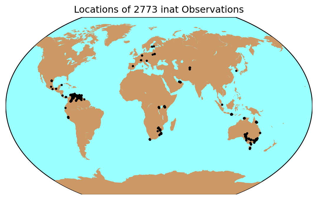
Step 3: Intersecting with Country and region Boundaries
We’ll overlay these observations on administrative boundaries using geopandas.
World Bank data
I found a link to these good quality data in the World Bank Group Data Catalog
zip_url='https://datacatalogfiles.worldbank.org/ddh-published-v2/0038272/3/DR0046659/wb_countries_admin0_10m.zip'
r = requests.get(zip_url)
z = zipfile.ZipFile(io.BytesIO(r.content))
for j in z.namelist():
    print(j)
WB_countries_Admin0_10m/
WB_countries_Admin0_10m/WB_countries_Admin0_10m.dbf
WB_countries_Admin0_10m/WB_countries_Admin0_10m.shp
WB_countries_Admin0_10m/WB_countries_Admin0_10m.shp.xml
WB_countries_Admin0_10m/WB_countries_Admin0_10m.prj
WB_countries_Admin0_10m/WB_countries_Admin0_10m.sbx
WB_countries_Admin0_10m/WB_countries_Admin0_10m.shx
WB_countries_Admin0_10m/WB_countries_Admin0_10m.cpg
WB_countries_Admin0_10m/WB_countries_Admin0_10m.sbnLoad the country boundaries from the web by combining the url to the zipfile and the file name within the zipfile:
shp_file = "WB_countries_Admin0_10m/WB_countries_Admin0_10m.shp"
remote_path = 'zip+{}!/{}'.format(zip_url, shp_file)

countries = gpd.read_file(remote_path)
And now intersect the data with a spatial join:
obs_with_countries = inat_obs_world.sjoin(countries, how='left')But wait, we have some observations unassigned to countries:
obs_with_countries.loc[obs_with_countries.WB_NAME.isna()]| longitude | latitude | location | species guess | url | attribution | geometry | index_right | OBJECTID | featurecla | ... | NAME_RU | NAME_SV | NAME_TR | NAME_VI | NAME_ZH | WB_NAME | WB_RULES | WB_REGION | Shape_Leng | Shape_Area | |
|---|---|---|---|---|---|---|---|---|---|---|---|---|---|---|---|---|---|---|---|---|---|
| 189 | -118.479683 | 33.993838 | Los Angeles County, US-CA, US | Rock Pigeon | https://inaturalist-open-data.s3.amazonaws.com... | (c) JR Ferrer-Paris, some rights reserved (CC BY) | POINT (-118.47968 33.99384) | NaN | NaN | NaN | ... | NaN | NaN | NaN | NaN | NaN | NaN | NaN | NaN | NaN | NaN |
| 190 | -118.479606 | 33.993770 | Los Angeles County, US-CA, US | House Sparrow | https://inaturalist-open-data.s3.amazonaws.com... | (c) JR Ferrer-Paris, some rights reserved (CC BY) | POINT (-118.47961 33.99377) | NaN | NaN | NaN | ... | NaN | NaN | NaN | NaN | NaN | NaN | NaN | NaN | NaN | NaN |
| 191 | -118.476596 | 33.990280 | Los Angeles County, US-CA, US | Western Gull | https://inaturalist-open-data.s3.amazonaws.com... | (c) JR Ferrer-Paris, some rights reserved (CC BY) | POINT (-118.4766 33.99028) | NaN | NaN | NaN | ... | NaN | NaN | NaN | NaN | NaN | NaN | NaN | NaN | NaN | NaN |
| 192 | -118.473123 | 33.986267 | Los Angeles County, US-CA, US | Hesperiini | https://inaturalist-open-data.s3.amazonaws.com... | (c) JR Ferrer-Paris, some rights reserved (CC BY) | POINT (-118.47312 33.98627) | NaN | NaN | NaN | ... | NaN | NaN | NaN | NaN | NaN | NaN | NaN | NaN | NaN | NaN |
| 193 | -118.472681 | 33.985681 | Los Angeles County, US-CA, US | None | https://inaturalist-open-data.s3.amazonaws.com... | (c) JR Ferrer-Paris, some rights reserved (CC BY) | POINT (-118.47268 33.98568) | NaN | NaN | NaN | ... | NaN | NaN | NaN | NaN | NaN | NaN | NaN | NaN | NaN | NaN |
| ... | ... | ... | ... | ... | ... | ... | ... | ... | ... | ... | ... | ... | ... | ... | ... | ... | ... | ... | ... | ... | ... |
| 3273 | 20.030967 | 60.207284 | Sund, Åland | ベニシジミ | https://inaturalist-open-data.s3.amazonaws.com... | (c) JR Ferrer-Paris, some rights reserved (CC BY) | POINT (20.03097 60.20728) | NaN | NaN | NaN | ... | NaN | NaN | NaN | NaN | NaN | NaN | NaN | NaN | NaN | NaN |
| 3274 | 19.943076 | 60.220928 | Finström, Åland | Ähriger Ehrenpreis | https://inaturalist-open-data.s3.amazonaws.com... | (c) JR Ferrer-Paris, some rights reserved (CC BY) | POINT (19.94308 60.22093) | NaN | NaN | NaN | ... | NaN | NaN | NaN | NaN | NaN | NaN | NaN | NaN | NaN | NaN |
| 3283 | 32.692072 | -28.296453 | Saint Lucia, South Africa | Humpback Whale | https://inaturalist-open-data.s3.amazonaws.com... | (c) JR Ferrer-Paris, some rights reserved (CC BY) | POINT (32.69207 -28.29645) | NaN | NaN | NaN | ... | NaN | NaN | NaN | NaN | NaN | NaN | NaN | NaN | NaN | NaN |
| 3285 | 32.565730 | -28.378646 | Saint Lucia, South Africa | Shy Albatross | https://inaturalist-open-data.s3.amazonaws.com... | (c) JR Ferrer-Paris, some rights reserved (CC BY) | POINT (32.56573 -28.37865) | NaN | NaN | NaN | ... | NaN | NaN | NaN | NaN | NaN | NaN | NaN | NaN | NaN | NaN |
| 3286 | -67.963415 | 10.495212 | Barrio de la Base Naval, Puerto Cabello 2050, ... | Blue Rainbow lizard | https://inaturalist-open-data.s3.amazonaws.com... | (c) JR Ferrer-Paris, some rights reserved (CC BY) | POINT (-67.96341 10.49521) | NaN | NaN | NaN | ... | NaN | NaN | NaN | NaN | NaN | NaN | NaN | NaN | NaN | NaN |
300 rows × 60 columns
We can improve this by using a join based on the nearest feature, but we will need to use an appropriate projection (for example the Eckert IV projection, ESRI:54012):
obs_with_countries = gpd.sjoin_nearest(
    inat_obs_world.to_crs("ESRI:54012"),
    countries.to_crs("ESRI:54012"),
    distance_col="distances",
    how="left")
ASGS structure
Since we have so many observations in Australia, we could break these down by regional areas. For example using the Australian Statistical Geographical Standard structure.
zip_url='https://www.abs.gov.au/statistics/standards/australian-statistical-geography-standard-asgs-edition-3/jul2021-jun2026/access-and-downloads/digital-boundary-files/SA2_2021_AUST_SHP_GDA2020.zip'
shp_file = "SA2_2021_AUST_GDA2020.shp"
Here we download and extract from the zipfile into our data folder, and then read the shapefile from this folder:
r = requests.get(zip_url)
z = zipfile.ZipFile(io.BytesIO(r.content))
z.extractall(repodir / "data")
australia = gpd.read_file(repodir / "data" / shp_file)
Use the join with the nearest feature but truncate to 50 km maximum distance:
obs_with_countries_and_regions = gpd.sjoin_nearest(
    obs_with_countries,
    australia.to_crs("ESRI:54012"),
    distance_col="distances",
    how="left",
    max_distance=50000,
    lsuffix='global',
    rsuffix='australia')
Let’s double check that observations with Australian regional data come from Australia, and if not, we will correct the country name:
An error here with GBR observations assigned to Fiji!
But now I have true obs from Fiji!
ss = obs_with_countries_and_regions.STE_NAME21.notna()
obs_with_countries_and_regions.loc[
    ss,
    "WB_NAME"].value_counts()
obs_with_countries_and_regions.loc[ss,
    "WB_NAME"] = "Australia"
And from which countries do the observations without Australian regional data come from?
obs_with_countries_and_regions.loc[
    obs_with_countries_and_regions.STE_NAME21.isna(),
    "WB_NAME"].value_counts()
WB_NAME Venezuela, Republica Bolivariana de 536 Indonesia 412 Mexico 343 South Africa 131 Colombia 117 Peru 103 United Arab Emirates 49 Rwanda 37 United States of America 35 Kenya 34 Tajikistan 33 Uganda 15 Panama 9 Finland 8 Poland 8 Costa Rica 6 Spain 4 Germany 4 Fiji 4 Italy 3 Belarus 3 Singapore 3 Ecuador 2 Switzerland 2 Trinidad and Tobago 2 Korea, Republic of 1 France 1 Guyana 1 Name: count, dtype: int64
Lots of observations from our trip to Bali and multiple visits to Monterrey!
We will need to fill in a placeholder value here to show these in the plot below:
obs_with_countries_and_regions.loc[
    obs_with_countries_and_regions.STE_NAME21.isna(),
    "STE_NAME21"] = "..."
Step 4: Interactive Graphs by Continent, Country, and Region
Finally, we’ll visualize the complete data using an interactive sunburst plot in plotly.
We start by grouping our data using continent, country and state and counting the number of unique species and places names.
aggfuncs = {'species guess':['count',pd.Series.nunique],
           'location':['count',pd.Series.nunique]}
colnames= ['CONTINENT','WB_NAME', # from Worldbank data
    'STE_NAME21'] # from ASGS data
obs_by_group=obs_with_countries_and_regions.groupby(colnames).agg(aggfuncs).reset_index()
obs_by_group.columns = [' '.join(col).strip() for col in obs_by_group.columns.values]
Now we create the plotly graph using this object. We can select to visualise data by number of unique species:
fig = px.sunburst(obs_by_group, path=colnames, values='species guess nunique', )
fig.show()
Or the count of observations based on locations:
fig = px.sunburst(obs_by_group, path=colnames, values='location count', )
fig.show()
And that’s it!
Conclusion
In summary, we:
- Downloaded observations with
pyinaturalist. - Mapped observations on a
basemapof the world. - Intersected observations with country and state boundaries using
geopandas. - Created insightful graphs with
plotly.
These steps transform field observations into engaging digital narratives, offering powerful ways to visualize biodiversity. Whether you’re a scientist, a digital cartographer, or a nature enthusiast, these tools can enhance your connection to the natural world.
Happy mapping and exploring! 🌍
Feel free to share your own mapping adventures or ask questions in the comments.
Footnotes
My alter ego in the iNat world↩︎