Visit to Darwin

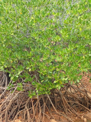
In July 2023 I visited Darwin for a Conference of the Ecological Society of Australia. During this trip I made some observations that I later uploaded to iNaturalist.

Since I just updated my entry for the visit to Hobart in January 2023, I thought it would be just as easy to adapt that code for the new dates, and get an updated travel log of this trip. So let’s adapt and adjust the code.

Tools and Libraries

Just as before, I will use my R skills to provide an overview of these observations of flora and fauna. Here is the list of R packages I will use:

library(rinat)
library(dplyr)
library(lubridate)
library(sf)
library(mapview)
library(leafpop)

• rinat: Access iNaturalist data with R.

• dplyr: A Grammar of Data Manipulation.

• sf: A package that provides simple features access for R.

• mapview: Interactive viewing of spatial data in R

Relative paths for files

I use the library here to manage relative paths of the project:

here::i_am("regions/Darwin-2023.qmd")

here() starts at /Users/z3529065/proyectos/CES/code-4-iNat

I save the downloaded inat data into this data folder at the root of the project folder:

if (!dir.exists(here::here("data")))
    dir.create(here::here("data"))
inat_obs_data <- here::here("data", "inat-obs.rds")

Query iNat

This will query all the observations from my iNaturalist user. I will save this to a data folder:

if (file.exists(inat_obs_data)) {
    user_obs <- readRDS(inat_obs_data)
} else {
    user_obs <- get_inat_obs_user("NeoMapas",maxresults = 5000) |> 
        mutate(dts=date(datetime), year=year(dts), month=month(dts))
    saveRDS(user_obs, inat_obs_data)
}

Filtering the data

For this post, I am focusing on the observation made between the 1 and the 8 of July 2023:

darwin_obs <- filter(user_obs, 
  dts %in% sprintf("2023-07-%02d", 1:8))

This is the number of observations that I have uploaded for those dates:

nrow(darwin_obs)

[1] 52

And this is the approximate number of species (or other taxa) included in those observations:

n_distinct(darwin_obs$species_guess)

[1] 43

Spatial attributes and map of locations

I can make this object spatially explicit using the function st_to_sf from package sf:

darwin_obs_xy <- st_as_sf(darwin_obs,
  coords=c("longitude","latitude"), 
  crs=4326)

We select only some columns to display in the map, and we jitter the coordinates slightly to display some overlapping points:

darwin_obs_xy <- select(darwin_obs_xy, 
  scientific_name,
  iconic_taxon_name,
  species_guess, 
  place_guess, 
  quality_grade,
  dts) |>
  st_jitter(amount = .005)

This example uses mapview to create a quick map with different layers for each day:

mapview(darwin_obs_xy,
    map.types = c("OpenStreetMap.DE", "Esri.WorldImagery"),
    zcol = "dts", burst = TRUE)

That is very handy to dig into the areas explored during this trip, use the controls to show or hide groups of observations and the buttons on the right side to zoom to a particular group.

Let’s make a gallery

First, I will prepare a template markdown string that includes a caption, a url for the image and attributes for displaying in a HTML document. Quarto uses the GLightbox javascript library so I just need to use the lightbox class.¹ I use the day of the observation as a group, so that photos of the same day can be shown as a carrousel.

photo_md_string <- "![*%s* observed in %s by %s@iNaturalist](%s){.lightbox group='day %s' height='150'}"

Now we populate these markdown strings using dplyr::mutate

darwin_obs <- darwin_obs |> 
  mutate(photo_md = sprintf(
    photo_md_string,
    species_guess, place_guess, user_login, image_url,
    dts))

Now, I want to breakdown the observations per day, let’s see how many there are for each day:

darwin_obs |> 
  group_by(date=dts) |> 
  summarise(
    obs=n(), 
    taxa=n_distinct(species_guess)) |>
    knitr::kable()

date	obs	taxa
2023-07-01	6	6
2023-07-02	16	14
2023-07-05	6	5
2023-07-07	12	11
2023-07-08	12	12

1 Jul

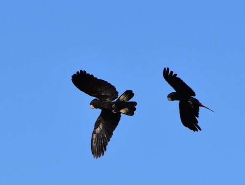
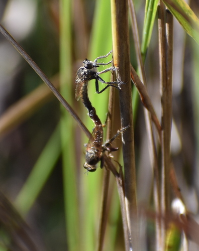
My first day exploring Darwin on foot.²

darwin_obs |> 
  filter(dts == "2023-07-01") |>
  pull(photo_md) |>
  cat()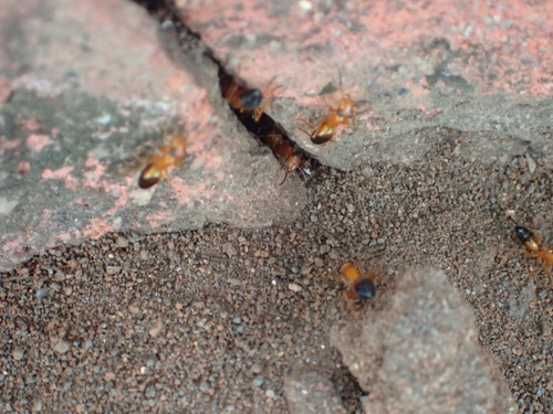

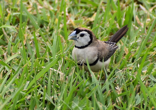
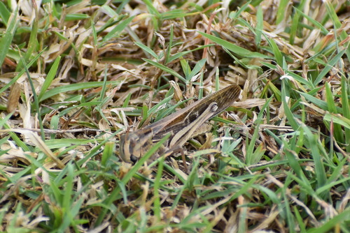
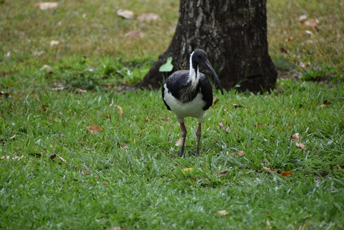
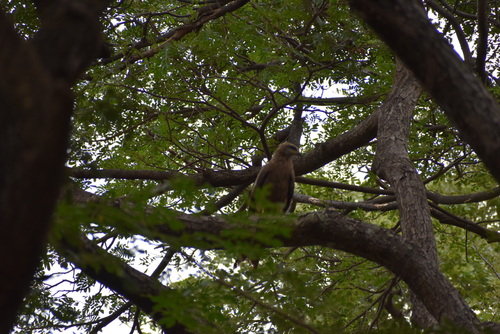
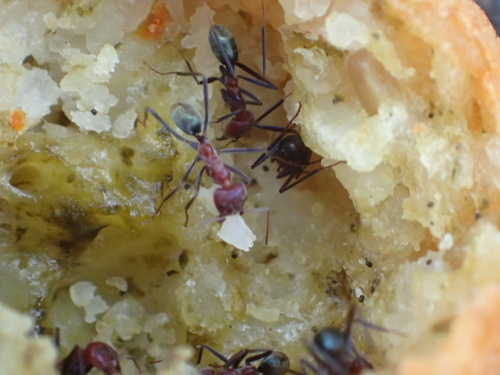
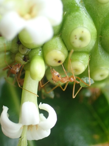
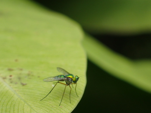
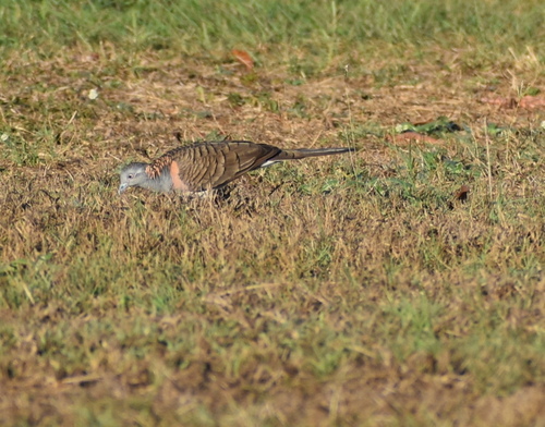
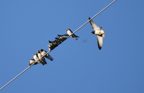
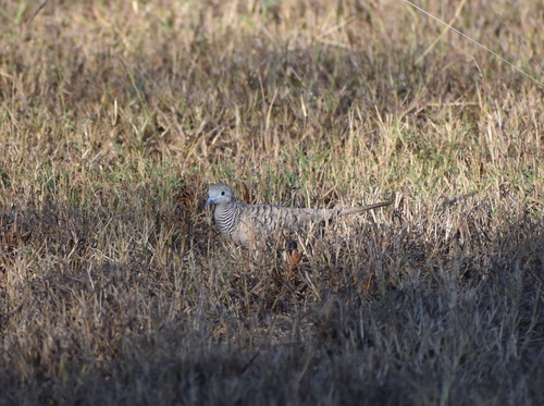
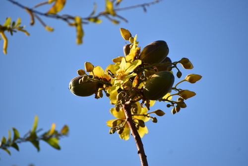
2 Jul

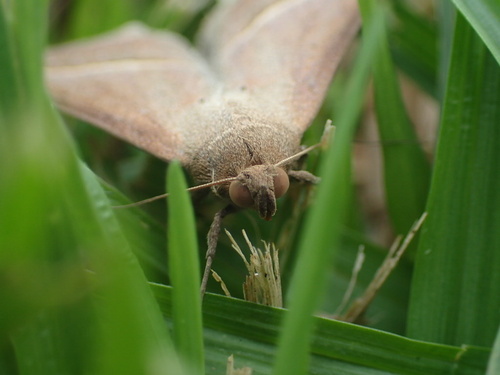
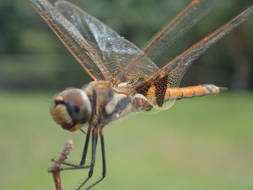
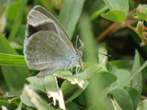
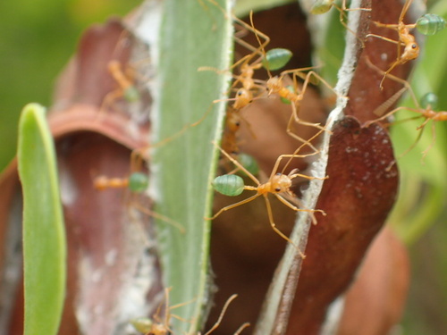
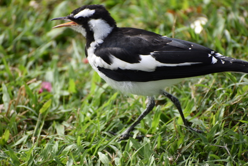
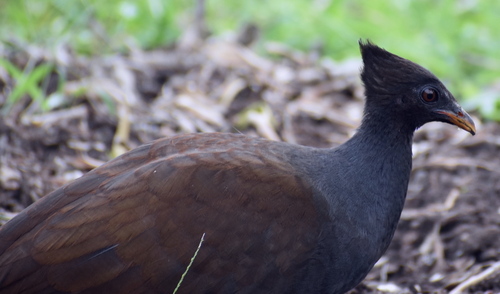
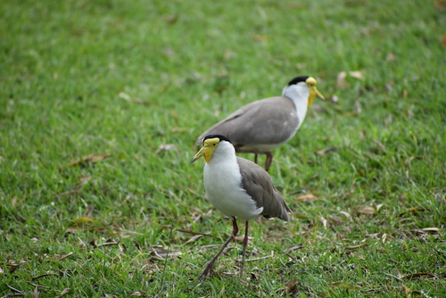
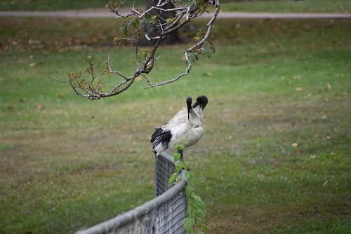
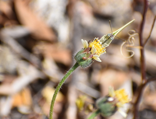
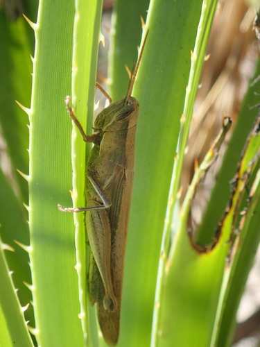
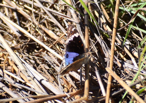
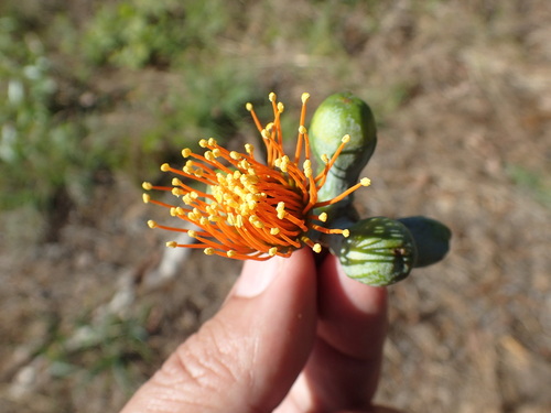
Exploring around the city before the conference get’s started. I walked around and got up to the Botanic Gardens.³

darwin_obs |> 
  filter(dts %in% "2023-07-02") |>
  pull(photo_md) |>
  cat()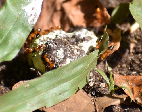

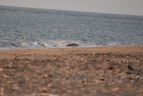
5 Jul

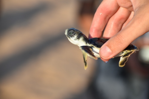
In the third day of the conference, I got into an excursion to Bare Sand Island to see Flatback Sea Turtles.⁴

darwin_obs |> 
  filter(dts %in% "2023-07-05") |>
  pull(photo_md) |>
  cat()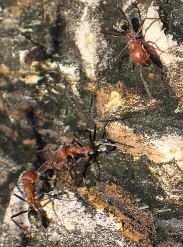

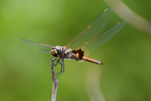
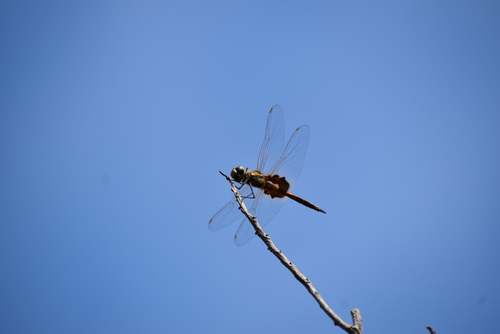
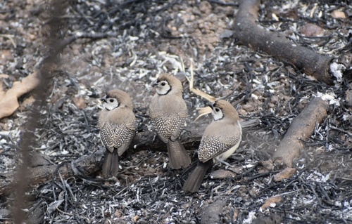
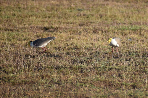
7 Jul

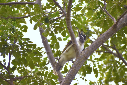
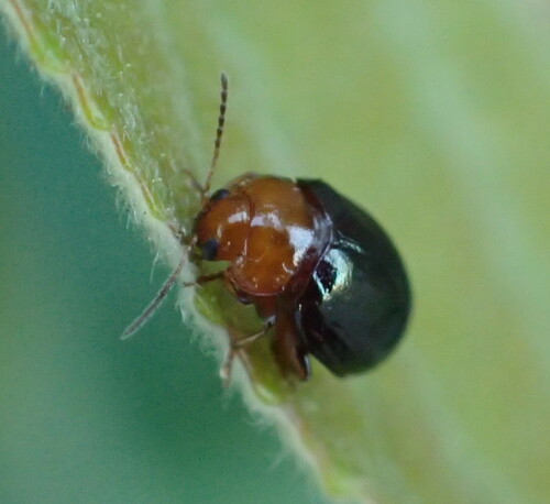
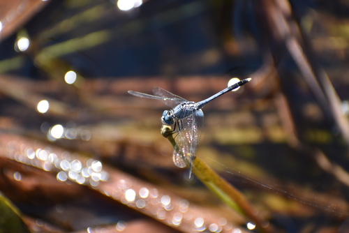
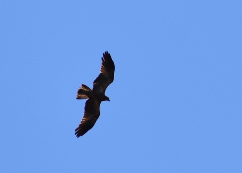
The conference is over, but I got to some extra activities around Darwin with more walks around the city and post-conference excursions.⁵

darwin_obs |> 
  filter(dts == "2023-07-07") |>
  pull(photo_md) |>
  cat()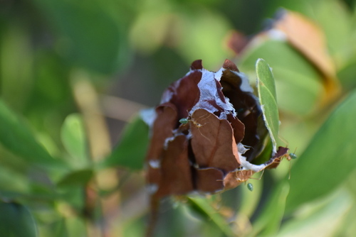

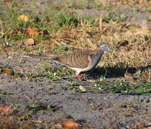
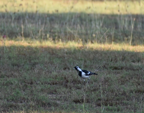
8 Jul

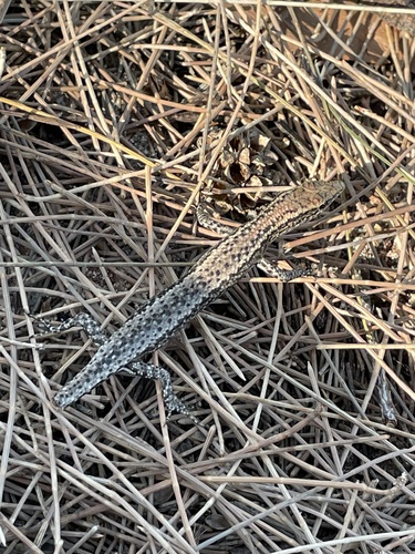
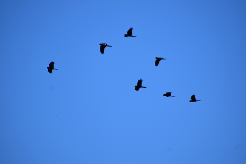
Went out with David to explore some sites around Girrawen.⁶

darwin_obs |> 
  filter(dts %in% "2023-07-08") |>
  pull(photo_md) |>
  cat()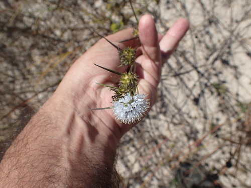

This is the end

That’s a fantastic summary of our trip! I hope you enjoyed and find the code useful. Cheers.

Session info

Here is the information for this R session:

sessionInfo()

R version 4.5.2 (2025-10-31)
Platform: aarch64-apple-darwin20
Running under: macOS Tahoe 26.3

Matrix products: default
BLAS:   /System/Library/Frameworks/Accelerate.framework/Versions/A/Frameworks/vecLib.framework/Versions/A/libBLAS.dylib 
LAPACK: /Library/Frameworks/R.framework/Versions/4.5-arm64/Resources/lib/libRlapack.dylib;  LAPACK version 3.12.1

locale:
[1] en_AU.UTF-8/en_AU.UTF-8/en_AU.UTF-8/C/en_AU.UTF-8/en_AU.UTF-8

time zone: Australia/Sydney
tzcode source: internal

attached base packages:
[1] stats     graphics  grDevices utils     datasets  methods   base     

other attached packages:
[1] leafpop_0.1.0   mapview_2.11.2  sf_1.0-24       lubridate_1.9.4
[5] dplyr_1.2.0     rinat_0.1.9    

loaded via a namespace (and not attached):
 [1] gtable_0.3.6            xfun_0.52               ggplot2_4.0.2          
 [4] raster_3.6-32           htmlwidgets_1.6.4       lattice_0.22-7         
 [7] leaflet.providers_2.0.0 vctrs_0.7.1             tools_4.5.2            
[10] crosstalk_1.2.1         generics_0.1.4          stats4_4.5.2           
[13] curl_7.0.0              tibble_3.3.1            proxy_0.4-29           
[16] pkgconfig_2.0.3         KernSmooth_2.23-26      satellite_1.0.5        
[19] RColorBrewer_1.1-3      S7_0.2.1                leaflet_2.2.2          
[22] uuid_1.2-1              lifecycle_1.0.5         compiler_4.5.2         
[25] farver_2.1.2            textshaping_1.0.1       terra_1.8-93           
[28] codetools_0.2-20        htmltools_0.5.8.1       maps_3.4.3             
[31] class_7.3-23            yaml_2.3.10             pillar_1.11.1          
[34] jquerylib_0.1.4         classInt_0.4-11         brew_1.0-10            
[37] tidyselect_1.2.1        digest_0.6.37           rprojroot_2.0.4        
[40] fastmap_1.2.0           grid_4.5.2              here_1.0.1             
[43] colorspace_2.1-2        cli_3.6.5               magrittr_2.0.4         
[46] base64enc_0.1-3         dichromat_2.0-0.1       leafem_0.2.4           
[49] e1071_1.7-17            withr_3.0.2             scales_1.4.0           
[52] sp_2.2-0                timechange_0.3.0        rmarkdown_2.29         
[55] httr_1.4.7              png_0.1-8               evaluate_1.0.3         
[58] knitr_1.50              rlang_1.1.7             Rcpp_1.1.1             
[61] glue_1.8.0              DBI_1.2.3               svglite_2.2.1          
[64] jsonlite_2.0.0          R6_2.6.1                plyr_1.8.9             
[67] systemfonts_1.2.3       units_1.0-0            

Footnotes

1. Check this posts’ source code for extra configuration details, and see the quarto documentation for instructions on how to activate this in your own quarto documents.

2. Check these observations in iNat

3. Check these observations in iNat

4. Check these observations in iNat

5. Check these observations in iNat

6. Check these observations in iNat