library(rinat)
library(dplyr)
library(lubridate)
library(sf)
library(mapview)
library(leafpop)Visit to Hobart
R
rinat
mapview
TAS
lightbox
In January 2023 I visited Hobart with my family. During this family holiday I made some observations that I later uploaded to iNaturalist.

Tools and Libraries
In this contribution I will use my R skills to provide an overview of these observations of flora and fauna. Here is the list of R packages I will use:
rinat: Access iNaturalist data with R.
dplyr: A Grammar of Data Manipulation.
sf: A package that provides simple features access for R.
mapview: Interactive viewing of spatial data in R
Relative paths for files
I use the library here to manage relative paths of the project:
here::i_am("regions/Hobart.qmd")here() starts at /Users/z3529065/proyectos/CES/code-4-iNatI save the downloaded inat data into this data folder at the root of the project folder:
if (!dir.exists(here::here("data")))
    dir.create(here::here("data"))
inat_obs_data <- here::here("data", "inat-obs.rds")
Query iNat
This will query all the observations from my iNaturalist user. I will save this to a data folder:
if (file.exists(inat_obs_data)) {
    user_obs <- readRDS(inat_obs_data)
} else {
    user_obs <- get_inat_obs_user("NeoMapas",maxresults = 5000) |>
        mutate(dts=date(datetime), year=year(dts), month=month(dts))
    saveRDS(user_obs, inat_obs_data)
}
Filtering the data
For this post, I am focusing on the observation made between the 17 and the 24 of January 2023:
hobart_obs <- filter(user_obs,
  dts %in% sprintf("2023-01-%s", 17:24))
This is the number of observations that I have uploaded for those dates:
nrow(hobart_obs)[1] 40And this is the approximate number of species (or other taxa) included in those observations:
n_distinct(hobart_obs$species_guess)[1] 35Spatial attributes and map of locations
I can make this object spatially explicit using the function st_to_sf from package sf:
hobart_obs_xy <- st_as_sf(hobart_obs,
  coords=c("longitude","latitude"),
  crs=4326)
We select only some columns to display in the map, and we jitter the coordinates slightly to display some overlapping points:
hobart_obs_xy <- select(hobart_obs_xy,
  scientific_name,
  iconic_taxon_name,
  species_guess,
  place_guess,
  quality_grade,
  dts) |>
  st_jitter(amount = .005)
This example uses mapview to create a quick map with different layers for each day:
mapview(hobart_obs_xy,
    map.types = c("OpenStreetMap.DE", "Esri.WorldImagery"),
    layer.name = c("Visit to Hobart"),
    zcol = "dts", burst = TRUE)
That is very handy to dig into the areas explored during this trip, use the controls to show or hide groups of observations and the buttons on the right side to zoom to a particular group.
Let’s make a gallery
First, I will prepare a template markdown string that includes a caption, a url for the image and attributes for displaying in a HTML document. Quarto uses the GLightbox javascript library so I just need to use the lightbox class.1 I use the day of the observation as a group, so that photos of the same day can be shown as a carrousel.
photo_md_string <- "{.lightbox group='day %s' height='150'}"Now we populate these markdown strings using dplyr::mutate
hobart_obs <- hobart_obs |>
  mutate(photo_md = sprintf(
    photo_md_string,
    species_guess, place_guess, user_login, image_url,
    dts))
Now, I want to breakdown the observations per day, let’s see how many there are for each day:
hobart_obs |>
  group_by(date=dts) |>
  summarise(
    obs=n(),
    taxa=n_distinct(species_guess)) |>
knitr::kable()| date | obs | taxa |
|---|---|---|
| 2023-01-18 | 18 | 15 |
| 2023-01-20 | 6 | 6 |
| 2023-01-21 | 1 | 1 |
| 2023-01-22 | 10 | 10 |
| 2023-01-23 | 4 | 3 |
| 2023-01-24 | 1 | 1 |
17 Jan
Arrival in Hobart, no observations uploaded today.
18 Jan
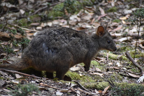
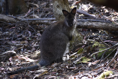
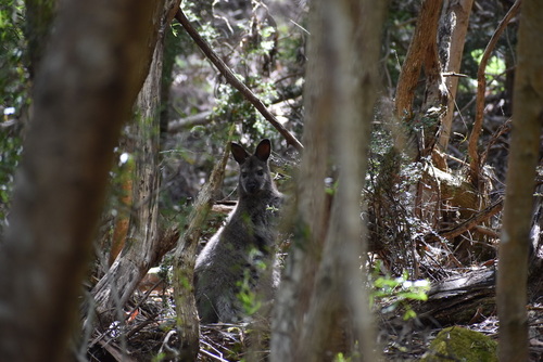
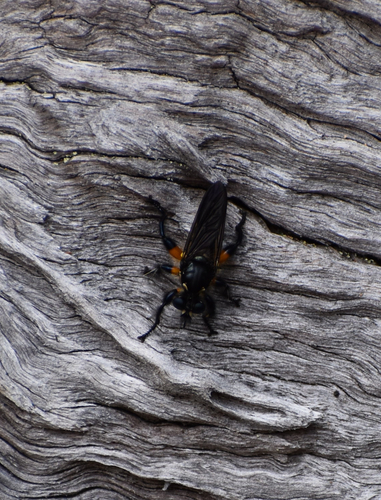
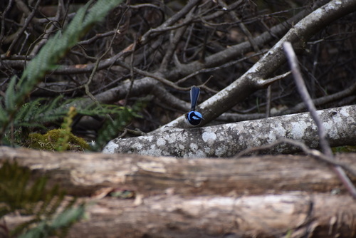
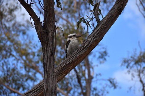
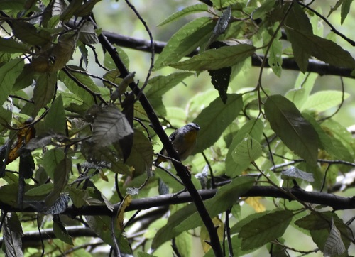
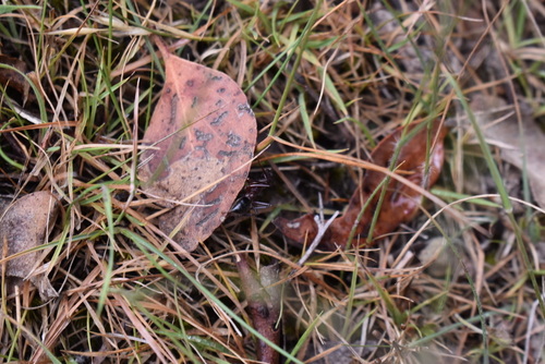
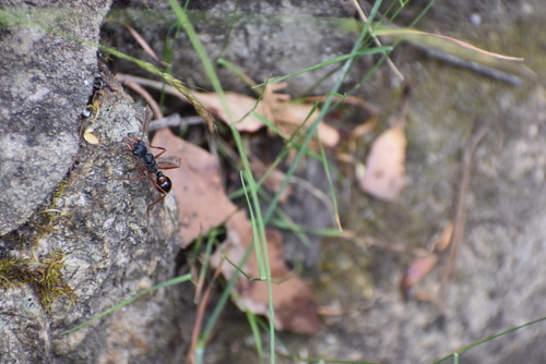
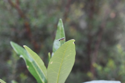
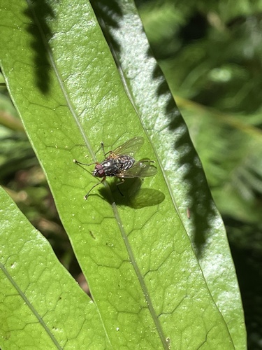
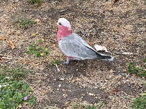
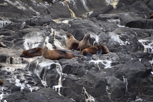
We started our trip with a walk through the Cascade Track in South Hobart. This track criss-crosses the Guy Fawkes Rivulet. Part of the track is on the Cascade Brewery land. We made a lot of family fotos, but I also pointed my camera to capture some interesting animals and plants. Abejandra was very excited when she spotted some cute macropods, and we also watched birds and some insects.

I got lots of observation this day, click on any photo to see a larger version with caption, then you can browse through the gallery using right or left arrows, hit the ESC key to exit the gallery.
hobart_obs |>
  filter(dts == "2023-01-18") |>
  pull(photo_md) |>
  cat()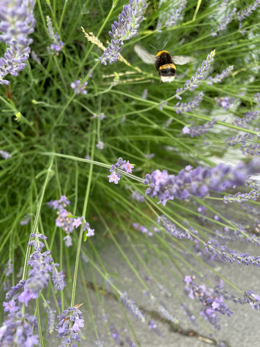
19 Jan
Walked around the city, explored the University campus, the Mawson’s Hutt Replica Museum, and the MONA.
No iNat observations this day.
20 Jan
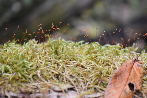
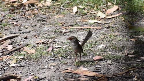
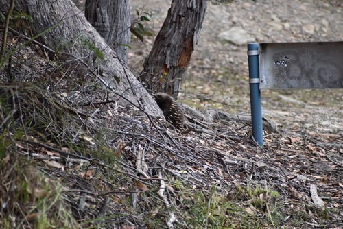
We started the day visiting Saint David’s Cathedral, then we went to walk some of the tracks in Wellington Park starting in Fern Glade, exploring O’Gradys Falls and other falls, caves and lookouts. Only a few observations uploaded so far.

hobart_obs |>
  filter(dts %in% "2023-01-20") |>
  pull(photo_md) |>
  cat()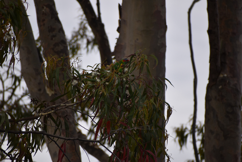
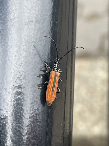
21 Jan
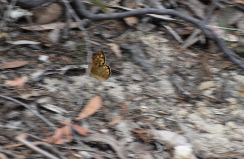
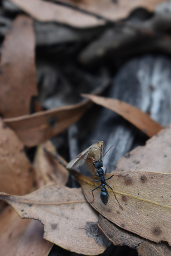
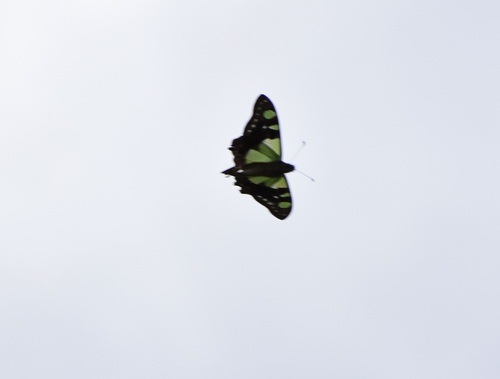
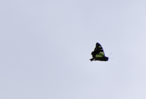
This day we explored the city and visited the Salamanca Markets and Tasmanian Museum and Art Gallery. I got at least one photo of a small butterfly while we were exploring the city.
hobart_obs |>
  filter(dts %in% "2023-01-21") |>
  pull(photo_md) |>
  cat()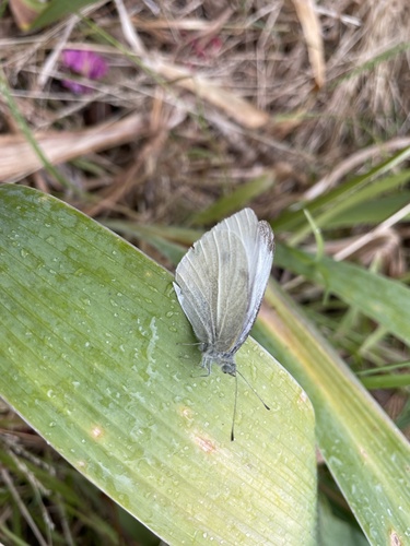
22 Jan
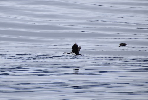
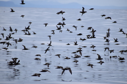
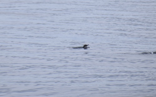
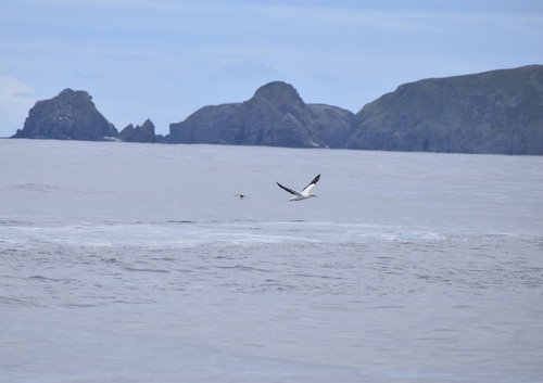
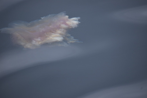
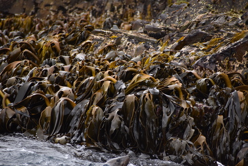
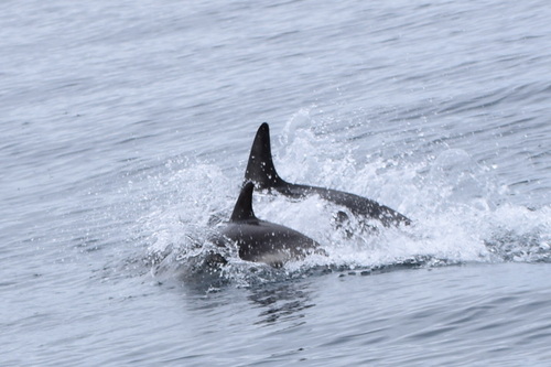
We booked a day trip to Bruny Island. We departed from Franklin Warf, we drove through the Neck and got on a boat to cruise around Adventure Bay and South Buny National Park.
I got a couple of shots of sealife on this day.
hobart_obs |>
  filter(dts == "2023-01-22") |>
  pull(photo_md) |>
  cat()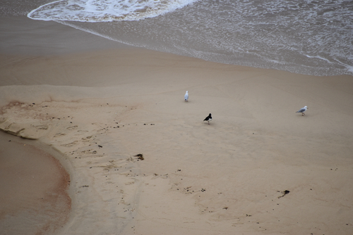
23 Jan
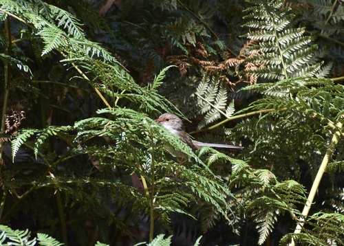
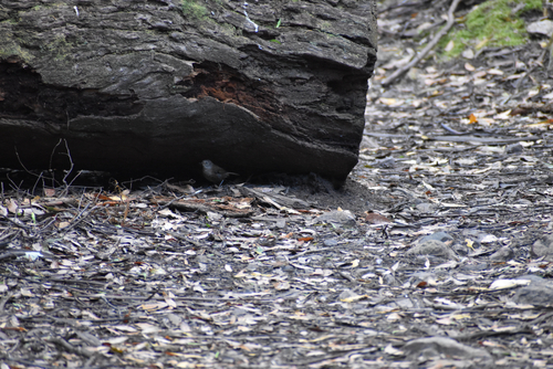
One more walk up Wellington Park, up to Sphinx Rock Lookout. A few observations on our way up and down.
hobart_obs |>
  filter(dts %in% "2023-01-23") |>
  pull(photo_md) |>
  cat()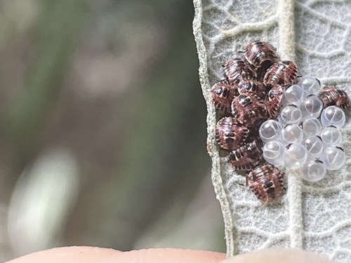
24 Jan
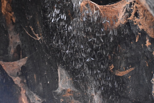
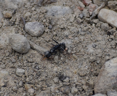
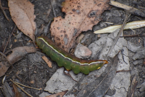
One last day before we flight back to Sydney. One last observation in iNat.

This day the kids had some fun in a bouncing park in the morning and in the afternoon we visited the Tasmanian Museum and Art Gallery once more. We spend the whole day in the city, but in some corner I found a small misterious insect larvae.
hobart_obs |>
  filter(dts %in% "2023-01-24") |>
  pull(photo_md) |>
  cat()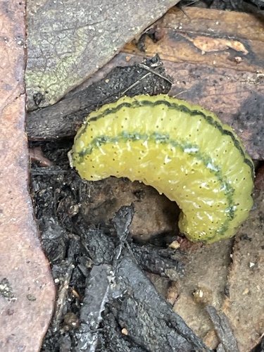
This is the end
That’s a fantastic summary of our trip! I hope you enjoyed and find the code useful. Cheers.
Session info
Here is the information for this R session:
sessionInfo()R version 4.5.2 (2025-10-31)
Platform: aarch64-apple-darwin20
Running under: macOS Tahoe 26.4.1
Matrix products: default
BLAS: /System/Library/Frameworks/Accelerate.framework/Versions/A/Frameworks/vecLib.framework/Versions/A/libBLAS.dylib
LAPACK: /Library/Frameworks/R.framework/Versions/4.5-arm64/Resources/lib/libRlapack.dylib; LAPACK version 3.12.1
locale:
[1] en_AU.UTF-8/en_AU.UTF-8/en_AU.UTF-8/C/en_AU.UTF-8/en_AU.UTF-8
time zone: Australia/Sydney
tzcode source: internal
attached base packages:
[1] stats graphics grDevices utils datasets methods base
other attached packages:
[1] leafpop_0.1.0 mapview_2.11.4 sf_1.1-0 lubridate_1.9.5
[5] dplyr_1.2.1 rinat_0.1.10
loaded via a namespace (and not attached):
[1] gtable_0.3.6 xfun_0.57 ggplot2_4.0.3
[4] raster_3.6-32 htmlwidgets_1.6.4 lattice_0.22-9
[7] leaflet.providers_3.0.0 vctrs_0.7.3 tools_4.5.2
[10] crosstalk_1.2.2 generics_0.1.4 stats4_4.5.2
[13] curl_7.1.0 tibble_3.3.1 proxy_0.4-29
[16] pkgconfig_2.0.3 KernSmooth_2.23-26 satellite_1.0.6
[19] RColorBrewer_1.1-3 S7_0.2.2 leaflet_2.2.3
[22] uuid_1.2-2 lifecycle_1.0.5 compiler_4.5.2
[25] farver_2.1.2 textshaping_1.0.5 terra_1.9-11
[28] codetools_0.2-20 htmltools_0.5.9 maps_3.4.3
[31] class_7.3-23 yaml_2.3.12 jquerylib_0.1.4
[34] pillar_1.11.1 classInt_0.4-11 brew_1.0-10
[37] tidyselect_1.2.1 digest_0.6.39 rprojroot_2.1.1
[40] fastmap_1.2.0 grid_4.5.2 here_1.0.2
[43] cli_3.6.6 magrittr_2.0.5 base64enc_0.1-6
[46] dichromat_2.0-0.1 leafem_0.2.5 e1071_1.7-17
[49] withr_3.0.2 scales_1.4.0 sp_2.2-1
[52] timechange_0.4.0 rmarkdown_2.31 httr_1.4.8
[55] otel_0.2.0 png_0.1-9 evaluate_1.0.5
[58] knitr_1.51 rlang_1.2.0 Rcpp_1.1.1-1.1
[61] glue_1.8.1 DBI_1.3.0 svglite_2.2.2
[64] jsonlite_2.0.0 R6_2.6.1 plyr_1.8.9
[67] systemfonts_1.3.2 units_1.0-1 Footnotes
Check this posts’ source code for extra configuration details, and see the quarto documentation for instructions on how to activate this in your own quarto documents.↩︎