Centre for Ecosystem Science, University of New South Wales
UNSW Data Science Hub, University of New South Wales
IUCN Commission on Ecosystem Management
Published
February 19, 2025
This document provides an example visualisation of the iNaturalist observations from the Gayini wetlands for the ARDC Gayini Trusted Environmental Data and Information Supply Chain project.
The Nari Nari Tribal Council manages and is actively restoring 80,000 ha of the extensive Gayini wetlands on the Murrumbidgee River. With their consortium partners, they are managing environmental flows, feral animals, cultural burning and grazing of livestock. The area is a key breeding area for waterbird rookeries, including the three ibis species, spoonbills, cormorants, herons and Australian pelicans. It also has extensive areas of lignum, river red gum and blackbox as well as terrestrial ecosystems. Nari Nari are supported by three other consortium partners, The Nature Conservancy, Murray Darling Wetlands Working Group and UNSW’s Centre for Ecosystem Science.
This document brings together data from online resources and is meant to be completely reproducible.
I will show here how to download information from a region in iNaturalist, query the observations in that region and visualise the data in three alternative ways: taxonomically, spatially, and temporally.
Reproducible workflow with Python
For this document I am using the get_observations function and the ICONIC_TAXA constants from PyiNaturalist for query and download of the data, Altair and Folium for data visualisation, and some functions from GeoPandas and pandas for convenience in reading data as a data frame, as well as selected functions from the urllib, owslib, json and datetime modules.
Load modules in python
from pyinaturalist import get_observations, ICONIC_TAXAimport altair as altimport foliumimport pandas as pdimport geopandas as gpdfrom datetime import datetimefrom owslib.wms import WebMapServiceimport urllib.parse, urllib.request, json from PIL import Imagefrom io import BytesIO
Data access and download
For this workflow we will load observations records and spatial data from iNaturalist and map layers from New South Wales Spatial Services and the Central Resource for Sharing and Enabling Environmental Data in NSW (SEED NSW).
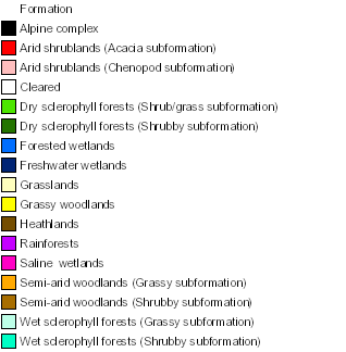
The spatial data for the Vegetation Formations and Classes of NSW Version 3.03 (Keith and Simpson 2012; updated in 2017) is available from the SEED portal. There are several access options documented in the metadata of the dataset, I use here the Web Map Service.
Vegetation Formations and Classes of NSW (version 3.03 - 200m Raster) - David A. Keith and Christopher C. Simpson. VIS_ID 3848. Updated in 2017 as version 3.1. Available from SEED data portal
The pyinaturalist library in Python provides convenient access to the iNaturalist API. We need the place_id that matches the area of interest to query the API with the function get_observations.
iNaturalist also provide access to the spatial information of places that have been contributed by the community. Here we construct a url to access the Gayini wetlands polygon in GeoJSON format.
The following snippet of code goes through the list of iNat’s observations (downloaded as a json object or, in this case, a python dictionary), and filters the research quality grade observations to extract records of species names, iconic taxon, date of the observation and the preferred common name, if present. We then summarise the observations grouped by species and count the total number of records per species.
Summarise observations by species
records =list()for obs in observations['results']:if obs['quality_grade'] =='research':if obs['taxon'] isnotNone: record = {'rank': obs['taxon']['rank'],'species_name': obs['taxon']['name'],'iconic_taxon': obs['taxon']['iconic_taxon_name'],'observed_on': datetime.date(obs['observed_on']), }if'preferred_common_name'in obs['taxon'].keys(): record['common_name']= obs['taxon']['preferred_common_name'] records.append(record)df = pd.DataFrame(records)colnames=['iconic_taxon','species_name','common_name','rank',]df.groupby(colnames)['species_name'].agg([ 'count'])
count
iconic_taxon
species_name
common_name
rank
Actinopterygii
Cyprinus carpio
European Carp
species
2
Gambusia holbrooki
Eastern Mosquitofish
species
1
Amphibia
Crinia parinsignifera
Beeping Froglet
species
1
Litoria peronii
Peron's Tree Frog
species
2
Ranoidea raniformis
Southern Bell Frog
species
4
Arachnida
Trichonephila edulis
Australian Golden Orbweaver
species
1
Aves
Anas gracilis
Grey Teal
species
1
Dromaius novaehollandiae
Emu
species
2
Melopsittacus undulatus
Budgerigar
species
1
Platalea regia
Royal Spoonbill
species
1
Tachybaptus novaehollandiae
Australasian Grebe
species
1
Insecta
Ecphantus quadrilobus
Crested Tooth-Grinder
species
1
Simosyrphus grandicornis
Yellow-shouldered Stout Hover Fly
species
1
Mollusca
Succinea australis
Southern Ambersnail
species
1
Plantae
Atriplex lindleyi
Lindley's Saltbush
species
1
Cirsium vulgare
Bull Thistle
species
1
Limonium lobatum
winged sea-lavender
species
1
Paspalum distichum
knot grass
species
1
Persicaria prostrata
Creeping Knotweed
species
1
Phyla nodiflora
turkey tangle frogfruit
species
1
Ptilotus nobilis
Yellow Tails
species
1
Sclerolaena brachyptera
Short-wing Copperburr
species
1
Sclerolaena muricata
Black Roly-poly
species
1
Trifolium resupinatum
Reversed clover
species
1
Reptilia
Chelodina longicollis
Eastern Snake-necked Turtle
species
1
Delma inornata
Olive Delma
species
1
Hemiaspis damelii
Grey Snake
species
3
Morelia spilota metcalfei
Inland Carpet Python
subspecies
1
Notechis scutatus
Tiger Snake
species
1
Pseudechis porphyriacus
Red-bellied Black Snake
species
3
Pseudonaja textilis
Eastern Brown Snake
species
1
Suta suta
Curl Snake
species
2
Underwoodisaurus milii
Thick-tailed Barking Gecko
species
2
Varanus varius
Lace Monitor
species
1
We can further group the species and observation by groups of iconic taxa.
iNaturalist group species into iconic taxa. Since we don’t need to get into the details of taxonomic classifications for this project, this will do for this excercise.
Map of iNat observations
For the spatial visualisation of the data, this code brings together the information from the NSW base map, the Terrestrial Vegetation map, the Gayini wetlands boundary polygon and the iNaturalist observations.
Make this Notebook Trusted to load map: File -> Trust Notebook
Legend for the vegetation map:
Show the code
display(vegmap_legend)
As the iNaturalist project has started recently, there is still a small number of observations that meet the research quality grade. Gayini is a great place to observe wildlife, but is also a remote place with few visitor uploading data to iNaturalist.
As the NNTC rangers are trained in the use of the iNat app, we expect to see an increase in the number of records and species detected.
The aim of this code is to be re-used and adapted to track the progress of the project.
About
Acknowledgement of country
I acknowledge the Bedegal and Gadigal peoples (Canberra) who are the Traditional Owners of the lands where UNSW Sydney is located, and the Nari-Nari who are the Traditional Custodians of the Gayini Wetlands.
Acknowledgement of funding
This work was supported by the Ian Potter Foundation and ARDC Gayini TEDISC project.
This document
This document was created with quarto, Jupyter, Python, and good quality coffee.
See the code tools in the top right corner of this document for all the source code, and the citation information at the bottom of this document.
@online{ferrer-paris2025,
  author = {Ferrer-Paris, José R.},
  title = {Reproducible Workflow for Visualisation of {iNaturalist}
    Observations in the {Gayini} Wetlands},
  date = {2025-02-19},
  url = {https://jrfep.quarto.pub/gayini-inat/},
  langid = {en}
}
For attribution, please cite this work as:
Ferrer-Paris, José R. 2025. “Reproducible Workflow for
Visualisation of iNaturalist Observations in the Gayini
Wetlands.” February 19, 2025. https://jrfep.quarto.pub/gayini-inat/.