Minimalistic basemaps

Have you ever needed a very simple background for your spatial data, but struggled to find a simple solution? I mean, interactive and multilayered maps are great for many applications. But sometimes we need something simple, a quick snapshot. Just enough detail to show the spatial context, something to find our bearings.

I have been experimenting with some solutions to this problem, and today I want to show how much we can do with the basemaps package in R.

I will illustrate this functionality by looking at some famous tropical glaciers around the world. I hope you will enjoy the journey.

`basemaps` library

basemaps is a lightweight R package with a very simple and straightforward objective: download or cache spatial basemaps from open sources. It can be used with some amazing resources like OpenStreetMap, Stamen, Stadia, Thunderforest, Carto, Mapbox, Esri and others. And the data is translated directly into the class you need: image, plot, spatial data, you name it.

So we start by loading the library:

library(basemaps)

And let’s also load other libraries we will need for the examples below:

library(sf)
library(dplyr)
library(ggplot2)
library(mapview)

Configuration

Although the basemaps library is very simple an sraightforward, sometimes it is useful to do some extra steps of configuration to optimise its use.

First, we can create a folder to cache the maps we download. If we skip this step, all intermediary files will be downloaded in a temporary folder and destroyed between sessions. Here are the lines of code I use to create my own folder for these files:

here::i_am("posts/basemaps-in-R/index.qmd")

here() starts at /Users/z3529065/proyectos/personal/spatial-one

my_map_dir <- here::here("sandbox")
if (!dir.exists(my_map_dir))
  dir.create(my_map_dir)

For some of the map providers you need to create an access token or API key before you can connect and download the data. I keep my tokens and api keys in a file called _environment.local, and I can read this file with:

readRenviron(here::here("_environment.local"))

Then, I can use the Sys.getenv function to retrieve the values stored there.

Lastly, I set default values for the basemaps package using set_defaults:

set_defaults(map_dir = my_map_dir,
  map_service = "osm_stadia", 
  map_type = "outdoors", 
  map_token = Sys.getenv("STADIA_API_KEY")
)

Where do we want to go?

Now we need to define our geographic region of interest. A bounding box, a point with a buffer or a geospatial object could be used to define a geographic extent.

Here we will use a vector file with the regional outlines of groups of tropical glaciers that I have shared in a OSF project.

Ferrer-Paris, J. R. (2024, February 21). Data for the global RLE assessment of Tropical Glacier Ecosystems. Retrieved from osf.io/432sb

Did you know you can read geopackage files from an url on the fly?, try this:

trop_glacier_groups <- read_sf("https://osf.io/download/nwdmf/")

Now we want to narrow down some groups, let’s try with the Sierra Nevada de Santa Marta in Colombia. We also need to project the data to the Web Mercator projection (EPSG: 3857) using the function st_transform.

glaciers_SNSM <- filter(trop_glacier_groups, 
    group_name == "Sierra Nevada de Santa Marta") |> 
    st_transform(crs=3857)

Basemap as an image

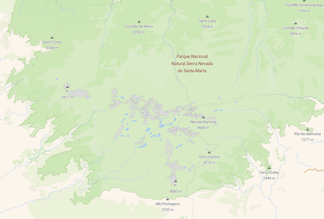
Using the function basemap_png we can get a nice basemap in a common image format. This can be stored in your computer for use in any document, or even as your screen background if you fancy that.

png_file <- basemap_png(glaciers_SNSM)

Using the function basemap_magick we can produce the same image file AND display it in out markdown documents using the underlying image magick functions. Remember that we have set default values for the map_dir, map_service, map_type and map_token parameters.

basemap_magick(glaciers_SNSM)

Loading basemap 'outdoors' from map service 'osm_stadia'...

Let go to a larger area

Now we want to go to a larger area, we will explore three clusters of glaciers in Ecuador. So again, we filter and project our spatial data:

glaciers_Ecuador <- filter(trop_glacier_groups, 
    country == "Ecuador") |> 
    st_transform(crs=3857)

Basemap in ggplot

Showing your data on top of a basemap can be very useful. If you use ggplot2 and want to add geospatial layers, you could use the basemap_gglayer function.

ggplot() + 
  basemap_gglayer(glaciers_Ecuador) +
  scale_fill_identity() + 
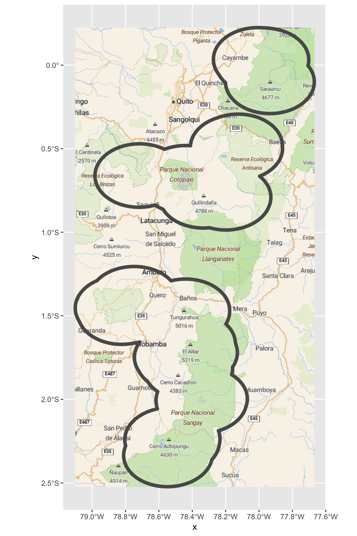
  geom_sf(data = glaciers_Ecuador, fill = NA, lwd = 2, alpha = .5)

Loading basemap 'outdoors' from map service 'osm_stadia'...
Using geom_raster() with maxpixels = 522522.

This basemap gives us some points of reference for the three groups of glaciers: the top group includes the glaciers near Cayambe, the middle one includes several peaks around Cotopaxi south of Quito, and the southern cluster follows a chain of mountain tops south of Ambato, including Tungurahua, El Altar and others. But given the static nature of the basemaps, they don’t always show what we want to highlight. For example the famous Chimborazo is omitted from this view. Maybe we do need to zoom and interact with our map afterall… 🤔

Try again with another zoom

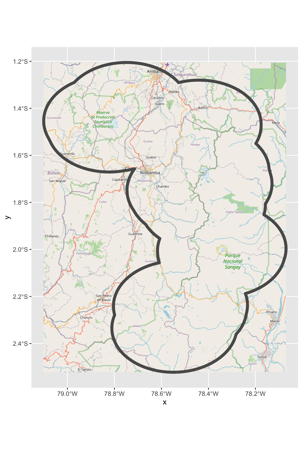
We can try with a different service and zooming to the southern cluster to get a better level of detail. We need to change the map_service and map_type parameters. We do not need the map_token parameter for some providers like OSM:

ggplot() + 
  basemap_gglayer(glaciers_Ecuador[1,], 
  map_service = "osm", 
    map_type = "streets") +
  scale_fill_identity() + 
  geom_sf(data = glaciers_Ecuador[1,], fill = NA, lwd = 2, alpha = .5)

Loading basemap 'streets' from map service 'osm'...
Using geom_raster() with maxpixels = 720209.

Ok, that looks very nice, but I had to try quite a few combinations. Basemaps are optimised to query maps at the zoom factor needed for the representation of the area of interest. So you always gets images of good resolution with a balanced level of detail.

Use the function get_maptypes() to see the available options.

Or let’s switch to interactivity again

But now, let’s go back to the interactivity question. Sometimes you can’t live without it. You can use basemaps in this context too. We will use the basemap_mapview function to overlay these static images on top of a dynamic map.

For example, let’s have a more “natural” background to see the majestic glaciers adorning the lush tropical landscape, let’s try changing the map_service and map_type parameters, and remember adding the value of your mapbox token for maps from mapbox.

basemap_mapview(glaciers_Ecuador,
    map_service = "mapbox", 
    map_type = "satellite", 
    map_token=Sys.getenv("MAPBOX_TOKEN")) +
    mapview(glaciers_Ecuador)

Loading basemap 'satellite' from map service 'mapbox'...

Now you can zoom in, zoom out, pan, select and activate/de-activate layers. So you can get the best of both worlds, or sort of.

Actually, there are other ways to combine these tiled basemaps in interactive views like mapview or leaflet, but I will explore that in another post.