Testing the redlistr package with examples from the Galápagos Islands

My colleagues and I have been working on a update to the R package called redlistr that aims to facilitate the process of calculating spatial metrics for the Red List of Ecosystem and Red List of Threatened Species assessments. In this post, I will share some examples of how we can use this package to analyse data from the Galápagos Islands, which are home to many unique species and ecosystems.

Package installation and loading

First, we need to install and load the redlistr package, along with some other packages that we will use for data manipulation and visualization.

If this is your first time using redlistr, you can install it from GitHub using a function from the devtools package. Make sure you have devtools installed and then run the following code:

## install.packages("devtools")
devtools::install_github("red-list-ecosystem/redlistr")

Once you have redlistr installed, you can load it along with other necessary packages:

library(redlistr)
library(dplyr)
library(ggplot2)
library(sf)
library(rgbif)
library(units)
library(ggrepel)

Since we are working with a package in active development, let’s check the version of the package redlistr that we have installed to ensure we are using the latest features and updates. You can do this by running the following code:

packageVersion("redlistr")

[1] '3.0.0'

I will also define a color palette that I will use for the visualizations in this post. This palette includes a range of colors that I find visually appealing and suitable for representing different elements in the maps and plots.

These colours are inspired by Guayasamín’s paintings like this one:

clrs <- c(
    "#995B4A", 
    "#584F4B",
    "#899B7A",
    "#D5B774",
    "#CC8956" )

Get a map of the Galápagos Islands

I found this map of the coastlines of the Galápagos Islands in the Galapagos Geoportal, which is a great resource for spatial data related to the Galápagos. The map is available as a GeoJSON file, which we can read into R using the sf package.

Thanks to the Charles Darwin Foundation!

This dataset has an Open Data Commons Open Database License / OSM (ODbL/OSM).

url <- "https://geodata.fcdarwin.org.ec/geoserver/ows?service=WFS&version=1.0.0&request=GetFeature&typename=geonode%3Agalapagos_island_project&outputFormat=json&srs=EPSG%3A4326&srsName=EPSG%3A4326"
galapagos_raw <- read_sf(url) 

Let’s have a glimpse of the data by looking at the first few rows:

glimpse(galapagos_raw)  

Rows: 398
Columns: 18
$ ogc_fid   <int> 1, 2, 3, 4, 5, 6, 7, 8, 9, 10, 11, 14, 12, 13, 15, 16, 17, 1…
$ id        <int> 1, 2, 3, 4, 5, 6, 7, 8, 9, 10, 11, 12, 13, 14, 15, 16, 17, 1…
$ gid       <int> 292, 338, 266, 201, 258, 302, 384, 335, 110, 216, 162, 108, …
$ tipo      <chr> "Roca", "Roca", "Roca", "Roca", "Roca", "Roca", "Islote", "R…
$ nombre    <chr> NA, NA, NA, NA, NA, NA, "Norte de Wolf", NA, "Santa Fé", NA,…
$ br_tipo   <chr> "Terrestre", "Terrestre", "Terrestre", "Terrestre", "Terrest…
$ bioregion <chr> "South-eastern/Centro Sur", "South-eastern/Centro Sur", "Sou…
$ br_code   <chr> "SE", "SE", "SE", "SE", "SE", "SE", "FN", "SE", "SE", "SE", …
$ gr_isla   <chr> "San Cristobal", "San Cristobal", "San Cristobal", "San Cris…
$ ig_code   <chr> "CB", "CB", "CB", "CB", "CB", "CB", "WO", "CB", "FE", "CB", …
$ code      <chr> "TSECB", "TSECB", "TSECB", "TSECB", "TSECB", "TSECB", "TFNWO…
$ area      <dbl> 2.079683e-01, 2.518432e-02, 2.858476e-03, 7.810453e-02, 5.41…
$ longitud  <dbl> 200.22101, 59.93381, 23.27626, 163.56060, 101.28358, 167.540…
$ map_code  <chr> NA, NA, NA, NA, NA, NA, "L", NA, "7", NA, NA, "39", NA, NA, …
$ raster    <int> 1, 1, 1, 1, 1, 1, 1, 1, 1, 1, 1, 1, 1, 1, 1, 1, 1, 1, 1, 1, …
$ zona      <chr> NA, NA, NA, NA, NA, NA, NA, NA, NA, NA, NA, NA, NA, NA, NA, …
$ isla      <chr> "Isabela", "Isabela", "Isabela", "Fernandina", "Isabela", "F…
$ geometry  <MULTIPOLYGON [°]> MULTIPOLYGON (((-91.36077 0..., MULTIPOLYGON ((…

This is a very detailed dataset, but we only need to focus on the groups of larger islands in the southern part of the Galápagos. I will show how to do that after we run some steps to prepare the spatial data.

Preparing the map for visualization

It is often advisable to validate the spatial data we have loaded to ensure that it is correctly formatted and does not contain any errors. We can use the st_is_valid() function from the sf package to check if the geometries in our dataset are valid. If we find any invalid geometries, we can use the st_make_valid() function to attempt to correct them. Here’s how you can do this:

# Check if all geometries are valid
all(st_is_valid(galapagos_raw))

[1] FALSE

# Make them valid
galapagos_valid <- st_make_valid(galapagos_raw)

For the next steps I will simplify the dataset by grouping features by the isla column. We will use the st_union() function from the sf package to combine the geometries of the features that belong to the same island group into a single geometry for each group.

galapagos_groups <- galapagos_valid |> 
    group_by(isla) |> 
    summarise(
        count=n(),
        area=sum(st_area(geometry)) |> 
        set_units('km2')) 

We can now check how many features we have in our dataset and how big they are. We can count the number of features and calculate their total area using some functions from dplyr and sf:

galapagos_groups |> 
    st_drop_geometry()|> 
    arrange(desc(area)) |>
    print(n=Inf)

# A tibble: 22 × 3
   isla          count       area
   <chr>         <int>     [km^2]
 1 Isabela         171 4732.     
 2 Santa Cruz       46  988.     
 3 Fernandina       62  648.     
 4 Santiago         30  579.     
 5 San Cristóbal    16  560.     
 6 Floreana         14  175.     
 7 Marchena          3  132.     
 8 Española         19   61.7    
 9 Pinta             4   59.7    
10 Baltra            1   25.4    
11 Santa Fe          4   24.6    
12 Pinzón            4   18.0    
13 Genovesa          1   13.8    
14 Rábida            3    4.98   
15 Seymour           1    1.91   
16 Wolf              4    1.31   
17 Darwin            9    0.689  
18 Daphne Mayor      2    0.337  
19 Bartolomé         1    0.200  
20 Mosquera          1    0.0783 
21 Daphne Menor      1    0.0586 
22 Roca Redonda      1    0.00973

The Galápagos are big, they include more than 20 groups of islands with a couple of them exceding the 100 square kilometers in area, and including several dozens of smaller features around the main landmasses.

Last, we want to make sure that the coordinate reference system (CRS) of our spatial data is correctly set. The CRS defines how the spatial data is projected and can affect how we calculate distances and areas. We can check the CRS of our dataset using the st_crs() function from the sf package:

st_crs(galapagos_groups)

Coordinate Reference System:
  User input: WGS 84 
  wkt:
GEOGCRS["WGS 84",
    DATUM["World Geodetic System 1984",
        ELLIPSOID["WGS 84",6378137,298.257223563,
            LENGTHUNIT["metre",1]]],
    PRIMEM["Greenwich",0,
        ANGLEUNIT["degree",0.0174532925199433]],
    CS[ellipsoidal,2],
        AXIS["geodetic latitude (Lat)",north,
            ORDER[1],
            ANGLEUNIT["degree",0.0174532925199433]],
        AXIS["geodetic longitude (Lon)",east,
            ORDER[2],
            ANGLEUNIT["degree",0.0174532925199433]],
    ID["EPSG",4326]]

The CRS is currently set to WGS 84 (EPSG:4326), which is a common geographic coordinate system. However, for certain analyses, especially those involving area calculations, it might be more appropriate to use a projected coordinate system that preserves area, such as UTM. We can transform our spatial data to a suitable projected CRS using the st_transform() function:

galapagos_projected <- st_transform(galapagos_groups, crs = 31977) # UTM zone 17S, which covers the Galápagos

Let’s make a quick plot to visualize the islands and ensure that our data looks correct. For visualisation purposes, I will exclude two small groups of islands, Darwin and Wolf, which are located in the north of the archipelago and are not relevant for our analysis.

galapagos_projected <- galapagos_projected |> 
    filter(!isla %in% c("Darwin", "Wolf")) 

We can use ggplot2 to create a simple map of the Galápagos Islands:

galapagos_plot <- ggplot() +
      geom_sf(data=galapagos_projected, 
        col=clrs[2],
        fill=clrs[3]
      ) +
      theme_bw()
      
galapagos_plot +
      geom_label_repel(data=galapagos_projected, aes(label=isla, geometry=geometry), stat = "sf_coordinates", size=5, alpha=0.5) 

Warning: ggrepel: 5 unlabeled data points (too many overlaps). Consider
increasing max.overlaps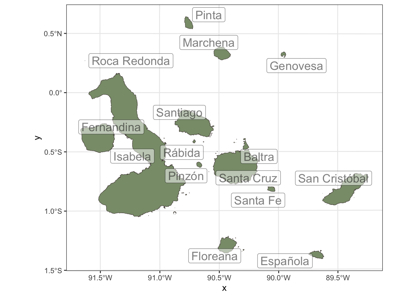

That’s great, but we are missing the most important part of the map: the species and ecosystems that we want to assess. In the next section, we will use the rgbif package to retrieve occurrence data for some of the species that are found in the Galápagos Islands, and then we will use redlistr to calculate spatial metrics for these species and their associated ecosystems.

Species occurrence data

I will focus on a couple of species that are endemic to the Galápagos Islands and are of conservation concern. For example, we can look at the Flightless Cormorant (Nannopterum harrisi) and the Scalesia forests formed by the Tree daisy (Scalesia pedunculata). We can use the rgbif package to retrieve occurrence data for these species from the Global Biodiversity Information Facility (GBIF).

Nannopterum harrisi

Nannopterum harrisi is endemic to the Galápagos Islands, Ecuador. It is found around most of the coast of Fernandina Island (mainly on the east), as well as on the north, northeast and west coasts of Isabela Island (Valle and Coulter 1987, H. Vargas and F. Cruz in litt. 2000).

We download the occurrence data for this species using the occ_search() function from the rgbif package. We will filter the results to include only those records that have coordinates, and we will set a high limit to try to retrieve as many records as possible.

target_taxon <- "Nannopterum harrisi"
taxon_occ <- occ_search(scientificName = target_taxon, 
    hasCoordinate = TRUE, 
    limit = 10000) 

We will convert the occurrence data into a spatial format using the sf package, and transform the coordinates to the same projected CRS that we used for the Galápagos map, so that we can perform spatial analyses and visualizations consistently.

n_harrisi <- taxon_occ$data |>
    st_as_sf(coords=c("decimalLongitude","decimalLatitude"), crs=4326) |>
    st_transform('EPSG:31977')

Scalesia pedunculata and the Scalesia forests

The Scalesia forest is a unique ecosystem found in the Galápagos Islands, characterized by the presence of the Tree daisy (Scalesia pedunculata). These forests are important for biodiversity and are also of conservation concern due to habitat loss and other threats.

I do not have a map of the Scalesia forests, but we can use occurrence data for Scalesia pedunculata as a proxy to understand the distribution of this ecosystem. We will follow a similar process as we did for Nannopterum harrisi to retrieve and prepare the occurrence data for Scalesia pedunculata.

target_taxon <- "Scalesia pedunculata"
taxon_occ <- occ_search(scientificName = target_taxon, hasCoordinate = TRUE, limit = 10000) 

s_pedunculata <- taxon_occ$data |>
    st_as_sf(coords=c("decimalLongitude","decimalLatitude"), crs=4326) |>
    st_transform('EPSG:31977')

Cleaning and filtering occurrence data

There are many occurrences records of these species, but many of those have inaccurate coordinates, so we will filter those out to ensure that our analysis is based on reliable data. I have to follow different approaches to filter the data for each species, because the quality of the records is different. For Nannopterum harrisi, we have a good number of records with accurate coordinates, so we can apply a simple filter based on the coordinateUncertaintyInMeters field to keep only those records that have a positional accuracy of less than 100 meters.

bb <- st_bbox(galapagos_projected)

n_harrisi <- n_harrisi |> 
    mutate(accuracy = if_else(coordinateUncertaintyInMeters < 1000, "Accurate", "Inaccurate", missing="Unknown"))

galapagos_plot +
      geom_sf(data=n_harrisi, aes(col=accuracy), size=2) +
      scale_color_manual(values=c(clrs[c(1,5,4)])) +
    coord_sf(xlim=c(bb[1], bb[3]), ylim=c(bb[2], bb[4]))+
    theme(legend.position = "top")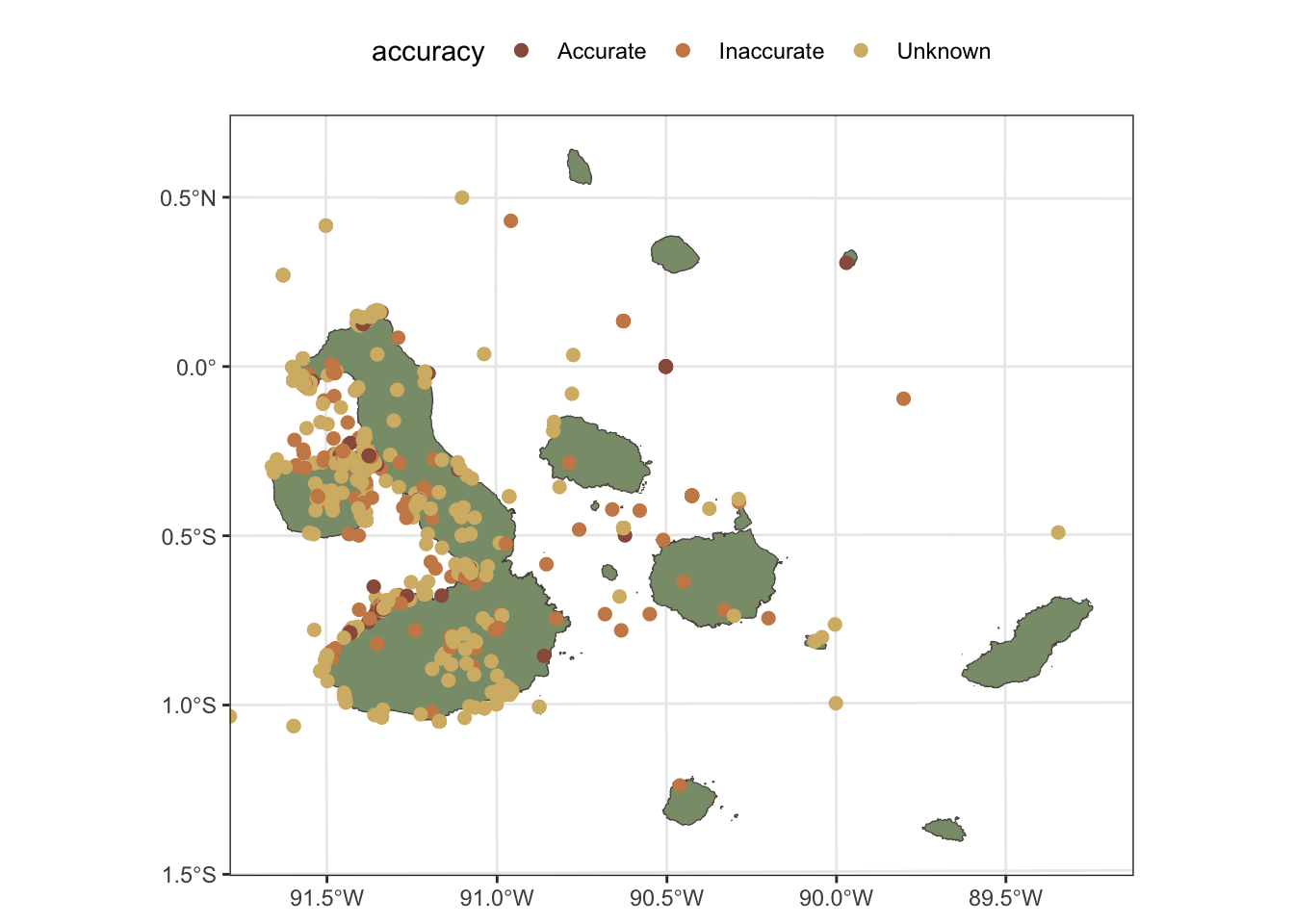

For Scalesia pedunculata, the situation is different, as the coordinates of the records have been obscured to protect the locations of this species, which is a common practice for sensitive species. In this case, we will not be able to filter the records based on positional accuracy, but we will filter these records to keep only those that are within the terrestrial parts of the Galápagos Islands. This allows us to still use the occurrence data to get an idea of the general distribution of the species and its associated ecosystem.

intersection_filter <- lengths(st_intersects(s_pedunculata, galapagos_projected)) == 1

s_pedunculata <- s_pedunculata |> 
    mutate(valid = if_else(intersection_filter, "On land", "On sea", missing="Unknown"))

galapagos_plot +
      geom_sf(data=s_pedunculata, aes(col=valid), size=2) +
      scale_color_manual(values=c(clrs[c(1,5,4)])) +
    coord_sf(xlim=c(bb[1], bb[3]), ylim=c(bb[2], bb[4]))+
    theme(legend.position = "top")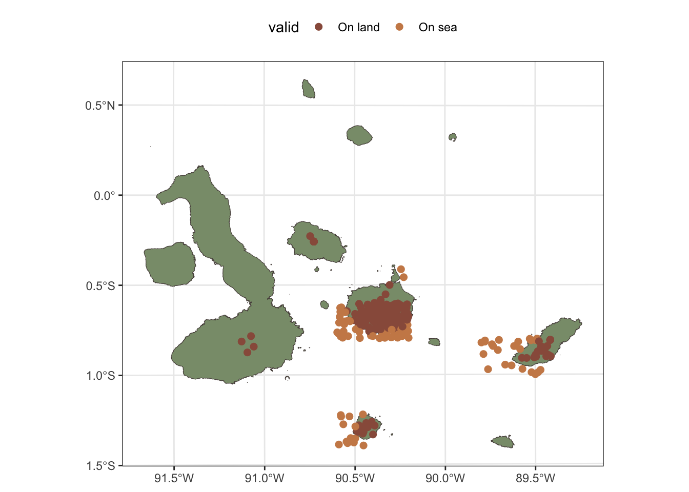

We will keep only those records that have a positional accuracy of less than 100 meters. We can use the coordinateUncertaintyInMeters field in the occurrence data to filter the records accordingly.

Calculating Extent of Occurrence (EOO)

We can calculate the Extent of Occurrence (EOO) for Nannopterum harrisi using the getEOO() function from the redlistr package. We will calculate the EOO for both the filtered dataset (with only accurate records) and the unfiltered dataset (including inaccurate records) to see how the inclusion of less accurate records affects the EOO calculation in this case.

taxon_EOO_all <- getEOO(filter(n_harrisi,accuracy %in% c("Accurate", "Inaccurate")))
summary(taxon_EOO_all)

Summary of EOO object
----------------------------
EOO area: 325,346.9 square kms
Polygon geometry type(s): POLYGON
Number of polygon features: 1
Input data class: sf
Input feature count: 474

taxon_EOO_filtered <- getEOO(filter(n_harrisi,accuracy=="Accurate"))
summary(taxon_EOO_filtered)

Summary of EOO object
----------------------------
EOO area: 14,558.8 square kms
Polygon geometry type(s): POLYGON
Number of polygon features: 1
Input data class: sf
Input feature count: 276

There is a huge difference between the EOO calculated with all records and the EOO calculated with only accurate records. This is because there are some inaccurate records that are located very far from the main landmasses of the Galápagos Islands, these are probably erroneous georeferences, dubious records or misidentified records, and they are inflating the EOO calculation. This highlights the importance of filtering occurrence data to get reliable outcomes in the assessment. Here we rely only on spatial filtering, but an expert based review of the records is recommended to identify and remove any records that are clearly erroneous or dubious, as well as to confirm the validity of the remaining records.

For Scalesia pedunculata we will calculate the EOO using only the records that are located on land, as these are the ones that are relevant for the distribution of this species and its associated ecosystem.

forest_EOO <- getEOO(filter(s_pedunculata, valid=="On land"))
summary(forest_EOO)

Summary of EOO object
----------------------------
EOO area: 12,869.51 square kms
Polygon geometry type(s): POLYGON
Number of polygon features: 1
Input data class: sf
Input feature count: 227

Calculating Area of Occupancy (AOO)

We calculate the Area of Occupancy (AOO) for Nannopterum harrisi using the getAOO() function from the redlistr package. We will use a grid size of 2000 meters, and we will not apply the bottom 1% rule but we will use jittering in this case.

taxon_AOO <- getAOO(
    filter(n_harrisi,accuracy=="Accurate"), 
    grid.size=2000, 
    bottom.1pct.rule = FALSE,
    jitter = TRUE)

Initialising grids

Assembling initial grids

Running jitter on units with 100 or fewer cells, n = 35

jittering  

This will give us a summary of the AOO calculation for this species. The AOO is calculated by counting the number of occupied cells and multiplying it by the area of each cell (in this case, 4 square kilometers). The AOO value can be used to assess the conservation status of the species, as it provides an estimate of the area that is currently occupied by the species and can help identify areas that are important for its conservation.

summary(taxon_AOO)

Class: AOO_grid
Number of grid cells: 40 
Grid extent:
      xmin       ymin       xmax       ymax 
 -685170.8  9903296.0  -501269.7 10035967.8 
CRS: SIRGAS 2000 / UTM zone 17S 

function call parameters:
grid size:  2000 
jitter:  TRUE 
n_jitter:  35 

The AOO value above is the minimum area that is occupied by the species, based on a sample of randomly placed grid of 2 km x 2 km cells. For each iteration we get a different AOO value, and we can see in the following stem-and-leaf plot that there is some spread in the AOO values across iterations. This is relevant to consider when using AOO values for assessment, as it highlights the uncertainty associated with this metric, which is influenced by the spatial distribution of the occurrence records.

stem(taxon_AOO@AOOvals)

  The decimal point is at the |

  40 | 0000
  42 | 00000000
  44 | 00000000000
  46 | 00000000
  48 | 000
  50 | 0

Now we will calculate the AOO for the Scalesia forests using the occurrence data for Scalesia pedunculata. We will use a grid size of 10,000 meters (10 km x 10 km cells), and we will not apply the bottom 1% rule but we will use jittering in this case.

forest_AOO <- getAOO(filter(s_pedunculata, valid=="On land"), 
    grid.size=10000, bottom.1pct.rule = FALSE, jitter = TRUE)

Initialising grids

Assembling initial grids

Running jitter on units with 100 or fewer cells, n = 35

jittering  

summary(forest_AOO)

Class: AOO_grid
Number of grid cells: 21 
Grid extent:
     xmin      ymin      xmax      ymax 
-642554.7 9850181.5 -439454.1 9984331.3 
CRS: SIRGAS 2000 / UTM zone 17S 

function call parameters:
grid size:  10000 
jitter:  TRUE 
n_jitter:  35 

stem(forest_AOO@AOOvals,scale=0.5)

  The decimal point is at the |

  20 | 0
  22 | 000000000000
  24 | 0000000000
  26 | 00000000000
  28 | 0

Visualising the results

Now we have the EOO and AOO calculated for Nannopterum harrisi, we can visualise these on the map of the Galápagos Islands. The EOO can be visualised as a polygon that represents the minimum convex hull that encompasses all the occurrence records, while the AOO can be visualised as a grid of cells that are occupied by the species.

galapagos_plot +
      geom_sf(data=taxon_AOO@grid, fill=clrs[4],col=clrs[1]) +
        geom_sf(data=taxon_EOO_filtered@pol, fill=NA, col=clrs[5], size=1)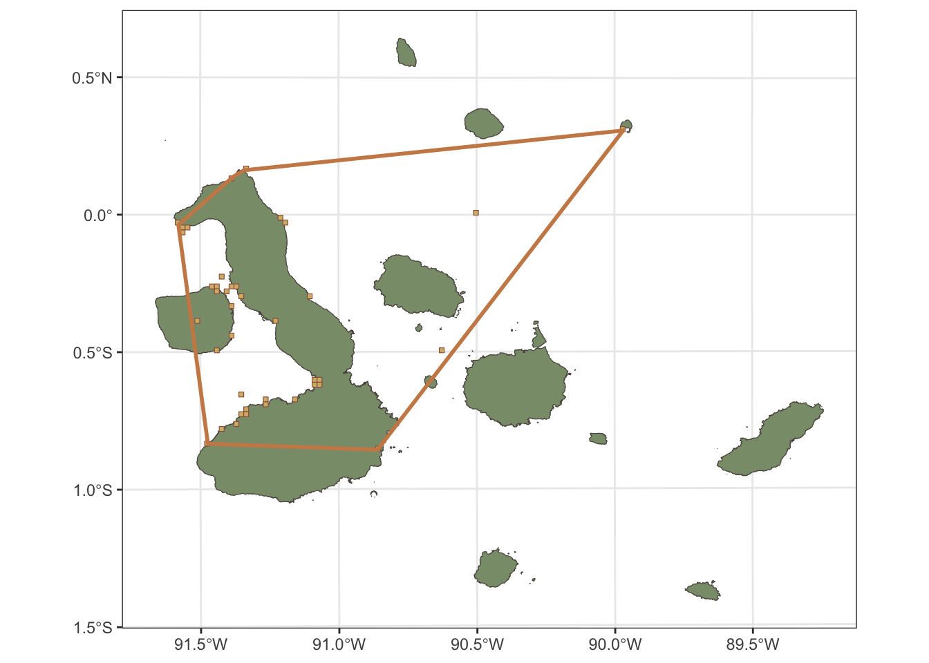

We do the same for the Scalesia forests, visualising the AOO as a grid of occupied cells and the EOO as a polygon that represents the minimum convex hull that encompasses all the occurrence records of Scalesia pedunculata. Here we are using larger grid cells for the AOO calculation, so the visualisation will show larger cells that are occupied by the species, which is more appropriate for an ecosystem-level assessment.

galapagos_plot +
      geom_sf(data=forest_AOO@grid, fill=clrs[4],col=clrs[1]) +
      geom_sf(data=forest_EOO@pol, fill=NA, col=clrs[5], size=1)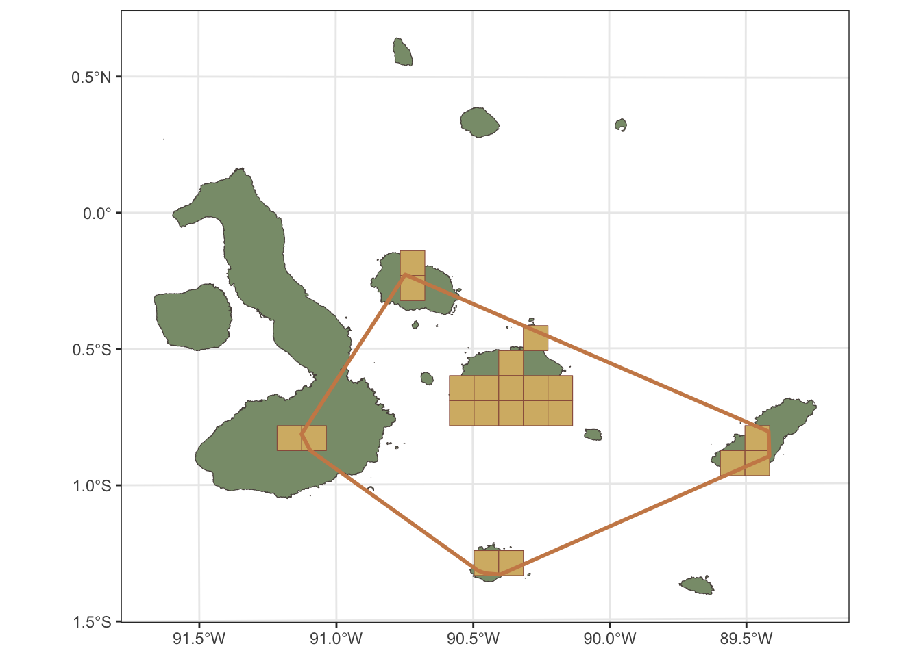

Is that it?

The EOO and AOO values are two of the spatial metrics that are used in the Red List of Threatened Species and the Red List of Ecosystems assessments. These metrics provide important information about the distribution and occupancy of the species and its associated ecosystem, but they are not sufficient to fully assess the conservation status of the species or ecosystem.

The spatial metrics need to be used in combination with an assessments of the threats that are affecting the species or ecosystem, as well as any trends in declines or degradation that are occurring. Moreover the full assessment involves many other criteria and subcriteria that need to be evaluates. For species this can be population size, population trends, habitat quality, and other factors that can influence the conservation status of the species. For ecosystems this can be declines in extent of the distribution, disruption of biotic processes or degradation of abiotic conditions.

You can see the results of the full assessment for Nannopterum harrisi in the IUCN Red List website, where it is currently listed as Vulnerable (VU) under criterion D2. The EOO and AOO values that we calculated in this post are twice as large as the values reported in the assessment, which are 5,900 km² for EOO and 50 km² for AOO. This might be due to an assessment based on a different set of occurrence records or a more accurate distribution map that excludes area temporarily used by the species or vagrant records. This highlights the importance of using reliable occurrence data and expert judgement in the assessment process, as well as the need to consider the uncertainty associated with the spatial metrics when making conservation decisions.

For the Scalesia forests, there is currently no assessment in the IUCN Red List of Ecosystems, but the EOO and AOO values that we calculated can provide useful information for a future assessment of this ecosystem, as they give an estimate of the distribution and occupancy of the ecosystem based on the occurrence data for Scalesia pedunculata.

You can find more information about the Red List of Threatened Species and the Red List of Ecosystems assessments in the IUCN Red List website and in the IUCN Red List of Ecosystems website. The redlistr package is a tool that can help with the calculation of spatial metrics, but it is not a substitute for a comprehensive assessment process that involves expert judgement and a thorough evaluation of all relevant criteria and subcriteria.