
import pandas as pd
import geopandas as gpd
from datetime import datetime
from pyinaturalist import (
    get_observations,
    get_taxa_by_id,
)
from IPython.display import display, HTML, Markdown
import contextily as cx
import matplotlib.pyplot as plt
import matplotlib.patches as patches
from matplotlib_scalebar.scalebar import ScaleBarWilsons Promontory National Park, Victoria
VIC
Python
pyinaturalist
contextily
Ada and I went to Melbourne to attend the 2024 ESA Conference (ESA2024) at the Melbourne Convention and Exhibition Centre from 9-13 December 2024. We signed up for one of the pre-conference tours to visit the famous Wilsons Promontory National Park.
After more than a year, I am finally uploading the observations I made during this trip and creating a travel journal with details for each day, including maps of the localities visited, quantitative summaries of observations, and some of the standout photos from my growing iNat collection.
Load Python modules
First I will load the necessary Python modules to help with data analysis and visualization.
These include pyinaturalist for all things iNatty, pandas and geopandas for data manipulation, contextily for the basemaps, matplotlib for plotting.
I will also need to set up relative paths to the data folders in this project using pyprojroot.
import pyprojroot
repodir = pyprojroot.find_root(pyprojroot.has_dir(".git"))
Download basemaps
I am going to download some basemaps for the areas I visited in Bali, so that I can overlay my observation points on them later. I am using a folder in the data directory to store these basemaps.
Since I use git for version control, and I don’t want to commit large files to it, this data folder needs to be in my .gitignore file.
basemap_dir = repodir / 'data' / 'basemapcache'
basemap_dir.mkdir(parents=True, exist_ok=True)
I select a few tiles from Open Street Map and CartoDB that cover the areas I visited, and download them using contextily. I am using to different providers to have some variety in the basemaps that I can use later.
slc_provider=cx.providers.OpenStreetMap.Mapnik
w, s, e, n = (146.2, -39.1, 146.5, -38.9)
prommap = cx.bounds2raster(w, s, e, n,
                     ll=True,
                     path=basemap_dir / "prom-map.tif",
                     source=slc_provider
)slc_provider=cx.providers.CartoDB.Positron
w, s, e, n = (146.2, -39.1, 146.5, -38.9)
tripmap = cx.bounds2raster(w, s, e, n,
ll=True,
path=basemap_dir / "prom-trip.tif",
source=slc_provider
)Download iNaturalist observations
Now this is one of those steps we are already familiar from other posts. First I check how many observations I have in iNaturalist from Bali during the trip dates.
observations = get_observations(user_id='NeoMapas',
                                d1="2024-12-05",
                                d2="2024-12-09",
                                per_page=0)
n_obs = observations['total_results']

# First we need to figure out how many observations to expect:
print("User NeoMapas has {} observations in this time frame".format(n_obs))
User NeoMapas has 125 observations in this time frameThen I download all the observations, including links to photos and metadata, using pyinaturalist.
Additionally, I download information about iconic taxonomic groups to help with later summaries and plots.
taxon_dict = get_taxa_by_id([3, 20978, 26036, 40151, 47115, 47158, 47126, 47157, 47170, 47178, 47224, 47792, 144128])I will go through these observations and extract the basic information I need for my summaries and plots.
records=list()
msg="Requesting observations from user NeoMapas: page {}, total of {} observations downloaded"
j=1
while len(records) < n_obs:
    print(msg.format(j,min(j*200,n_obs)))
    observations = get_observations(
        user_id='NeoMapas',
        d1="2024-12-05",
        d2="2024-12-09",
        per_page=1000,
        page=j)
    for obs in observations['results']:
        record = {'quality': obs['quality_grade'],
        'description': obs['description'],
        'location': obs['place_guess'],
        'geoprivacy': obs['taxon_geoprivacy'],
        'longitude': obs['location'][1],
        'latitude': obs['location'][0],
        'species guess': obs['species_guess'],
        'Fecha': obs['observed_on'],
        'points': obs['faves_count'] * 10 + obs['comments_count'] + obs['identifications_count'] * 3,
        }
        if len(obs['observation_photos'])>0:
            record['url'] = obs['observation_photos'][0]['photo']['url'].replace('square', 'medium')
            record['attribution'] = obs['observation_photos'][0]['photo']['attribution']
        record['groups'] = [x['name'] for x in taxon_dict['results'] if x['id'] in obs['taxon']['ancestor_ids']]
        records.append(record)
    j=j+1
Requesting observations from user NeoMapas: page 1, total of 125 observations downloadedThis goes now into a pandas DataFrame for easier manipulation.
df=pd.DataFrame(records)And a GeoDataFrame for mapping.
inat_obs=gpd.GeoDataFrame(
    df,
    geometry=gpd.points_from_xy(df.longitude, df.latitude),
    crs=4326
).to_crs(epsg=3857)
And before I forget, lets reformat the observation dates into simple strings for easier filtering.
inat_obs["dia"]=inat_obs.Fecha.apply(datetime.date).apply(lambda x: str(x))Map of observations
I can plot these observations on a map to highliht the locations I visited (gray circles on the map). I am using here a static basemap instead of the interactive one used in the previous posts.
Notice that all my observations were made in the southern part of Bali, where we spent our time during this trip (red rectangle).
fig, ax = plt.subplots(1, 1)
fig.set_size_inches(10,10)

inat_obs.plot(
    ax=ax,
    facecolor='grey',
    alpha=0.7,
    edgecolor='black',)

cx.add_basemap(
    ax,
    crs=inat_obs.crs,
    source = basemap_dir / "prom-map.tif",
    reset_extent=False
)

ax.add_artist(ScaleBar(1))
plt.show()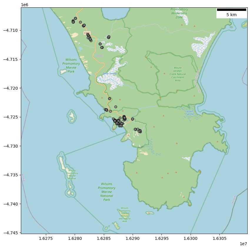
One advantage of using a static basemap is that we can easily save the map as a high-resolution image for later use. In this case, I will be zooming in to that red rectangle and using a different base layer to give a different look. I will highlight the observation points for each day to make them stand out against the basemap and the observations from the rest of the trip. Since I need to do this for each day, it is best to define a function that can be reused multiple times:
def mapday(day):
    fig, ax = plt.subplots(1, 1)
    inat_obs.plot(
        ax=ax,
        facecolor='grey')
    ss = (inat_obs.dia == day) & (inat_obs.geoprivacy != 'obscured')
    inat_obs.loc[ss].plot(
        ax=ax,
        facecolor='magenta',
        edgecolor='cyan')
    cx.add_basemap(
        ax,
        crs=inat_obs.crs,
        source = basemap_dir / "prom-trip.tif",
        reset_extent=False
    )
    #plt.xlim((1.28e7, 1.287e7))
    #plt.ylim((-9.95e5, -9.35e5))
    plt.show()
I am also defining a function to summarise the number of observations per day. This function uses Mardown and HTML to format the output nicely and provide a text description of the observations made on each day, including the total number, the numbers per iconic group and a preview of the more interesting observations of the day (selected by the numbers of favorites, ids and comments).
def summarise_obs(day):
df = inat_obs.loc[inat_obs.dia==day]
best = df.sort_values('points', ascending=False).head(3)
best['species guess'] = best['species guess'].fillna('-- unassigned --')
bestguess=', '.join(best['species guess'].to_list())
urls = best['url'].to_list()
total = df.shape[0]
group_counts = df['groups'].explode().value_counts()
groupstr= ', '.join([f"{count} {item}" for item, count in group_counts.items()])
display(Markdown(f"So far I have uploaded a total of %s observations. With %s tentatively identified at different taxonomic levels. The three more interesting observations so far are %s." % (total, groupstr, bestguess )))
display(HTML("".join([f"<img src='{url}' height=150> " for url in urls])))
display(Markdown("Check all the observations [here](https://www.inaturalist.org/observations?place_id=any&user_id=NeoMapas&d1=%s&d2=%s){target='inat'}" % (day,day)))Travel log
Now here is where my travel log begins. For each day of the trip, I will provide a summary of the observations made, including the map, the quantitative summary and some of the standout photos.
Day 1: Thursday 5 December
10:00 am departure from Melbourne. 2:00 pm Arrived at Wilsons Promontory National Park, attending two presentations: 2:00 pm Introduction to the landscape ecology, geomorphology and fire history of the northern section of the park, and 8:00 pm Introduction to the ecology of Wilsons Promontory and some of its fire management challenges.
day='2024-12-05'
mapday(day)
summarise_obs(day)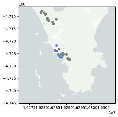
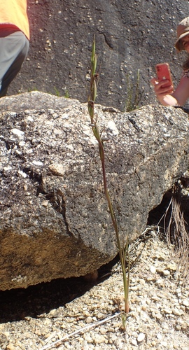
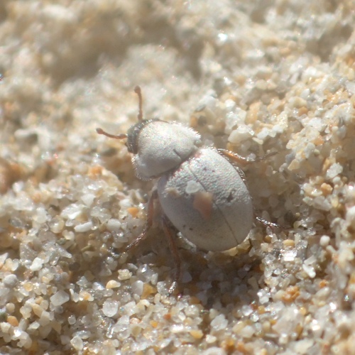
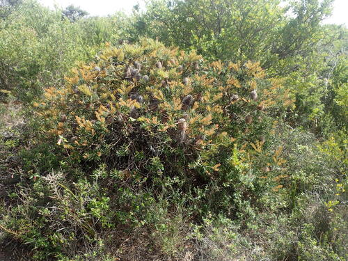
So far I have uploaded a total of 8 observations. With 3 Plantae, 1 Insecta, 1 Fungi tentatively identified at different taxonomic levels. The three more interesting observations so far are Birds mouth orchid, Phycosecis, Butterfly Bush.
Check all the observations here
Day 3: Friday 6 December
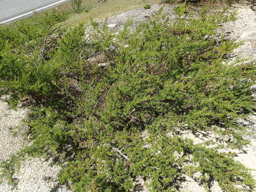
The morning was spent exploring the challenges of managing heathlands in the face of rapid invasion by Coast Tea-tree. We walked from Tidal River through recently burnt heathlands to the Lilly Pilly Gully carpark and then over Tidal Overlook to inspect the impact of recent management actions, before returning to accommodation at Tidal River for lunch (length of walk 5.4 km, moderate grade).
We received an introduction talk to the challenges of managing tall wet forests in a landscape that has suffered from too frequent fires; creating ‘landscape traps’.
We walked 0.5 km to a lookout on Mt Oberon to view affected areas and discuss management strategies in an era of climate change.
day='2024-12-06'
mapday(day)
summarise_obs(day)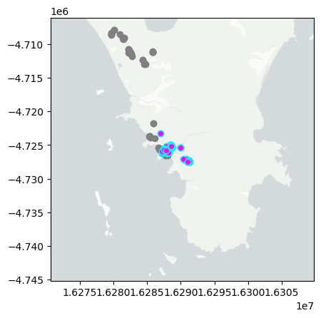
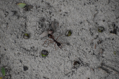
So far I have uploaded a total of 53 observations. With 25 Insecta, 15 Plantae, 13 Aves, 10 Lepidoptera, 9 Papilionoidea tentatively identified at different taxonomic levels. The three more interesting observations so far are Jack Jumper Ant, Triggerplants, Rosy Hyacinth Orchid.
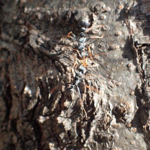
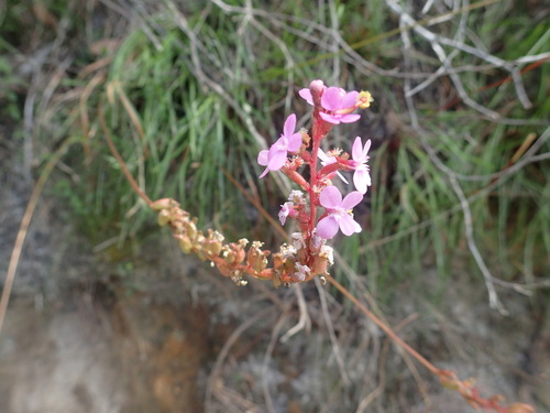
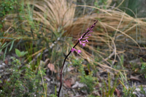
Check all the observations here
Day 4: Saturday 7 December
The morning was spent gaining an understanding of the role of fire and herbivore control in managing invasion of Coastal Grassy Woodlands by Coast Tea-tree and Coast Wattle, and restoration of grasslands in the northern section of the park.
We explored the challenges of sand heathland conservation action involving combined application of mechanical mulching of invasive Coast Tea-tree, followed by prescribed fire.
We visited examples of healthy heathland along the Five Mile Track and inspected tea-tree invaded sites at which both mulching and fire treatments have been applied along the Airstrip Firebreak.
day='2024-12-07'
mapday(day)
summarise_obs(day)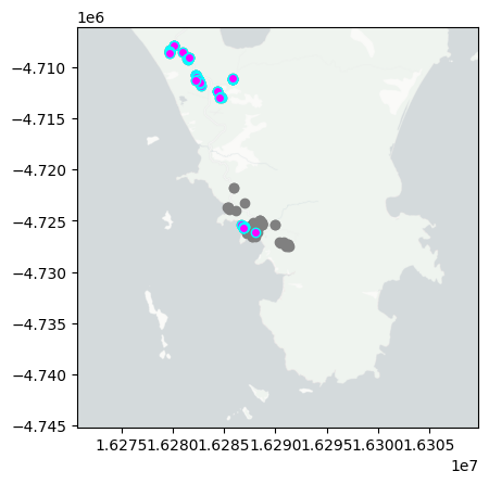
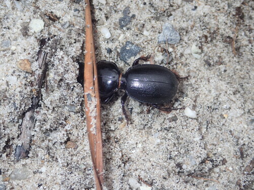
So far I have uploaded a total of 57 observations. With 24 Plantae, 16 Aves, 6 Insecta, 3 Mammalia, 2 Mollusca, 2 Reptilia, 1 Myriapoda tentatively identified at different taxonomic levels. The three more interesting observations so far are Beach Spinifex, Bare-nosed Wombat, Black-scaped Bull ant.
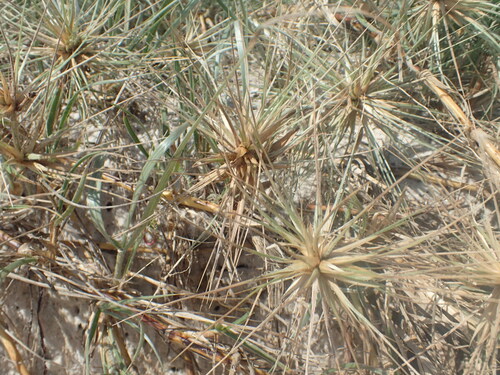
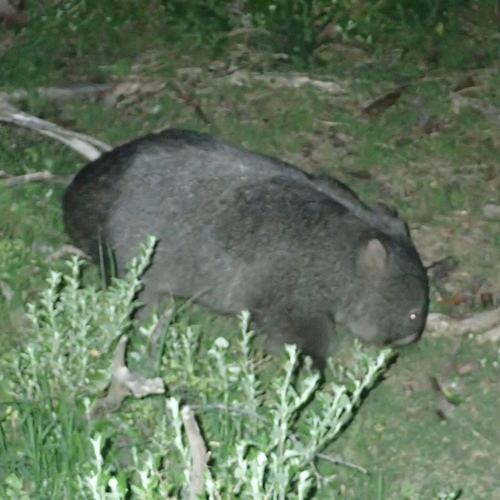
Check all the observations here
Day 5: Sunday 8 December
Morning stop in two beach sites, then driving back to Melbourne.
day='2024-12-08'
mapday(day)
summarise_obs(day)
So far I have uploaded a total of 7 observations. With 4 Plantae, 1 Insecta tentatively identified at different taxonomic levels. The three more interesting observations so far are Crystal Jellies, Scaraphites rotundipennis, Plants.
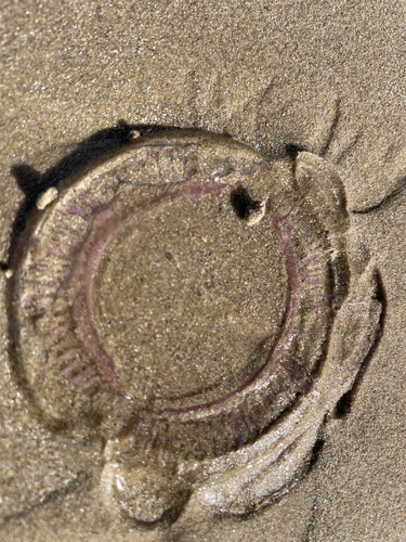
Check all the observations here
And this is the end of our trip!
So nice to revisit these memories and share some of the fotos I took during the trip.
I found that this code helped me to find a a nice and reproducible way to document my observations and combine these with notes of my experiences during the trip. I hope you enjoyed reading about it, that you find the photos interesting and that the code is useful for other.
I still have many more fotos to upload to iNaturalist, so stay tuned for more updates in the future!