From observation to record creation

Python

seaborn

statsmodels

Author

José R. Ferrer-Paris

Published

August 30, 2025

Modified

February 23, 2026

I have been occasionally uploading observations into iNaturalist since 2015, but it is only in recent years (since 2022) that I have been picking up some tricks and tools to do this in a regular basis.

I have already explored the temporal patterns of my observation effort throughout the years. Here I want to show the patterns in the creation of records.

Particularly I will explore:

the cross-tabulation of year of observation with the year of record creation (upload),
which iconic taxa were more popular in different years, and
which tools were used to upload records over time.

As a bonus I will throw in some nice graphics!

Import libraries

from pyinaturalist import get_observations
import pandas as pd
from IPython.display import display, Markdown
import seaborn as sns
import matplotlib.pyplot as plt
from statsmodels.graphics.mosaicplot import mosaic

Download records

First we need to figure out how many observations to expect:

username = 'neomapas'
observations = get_observations(user_id=username, per_page=0)
n_obs = observations['total_results']
print("User _{}_ has {} observations in iNaturalist".format(username,n_obs))

User _neomapas_ has 2644 observations in iNaturalist

Now we use the pagination trick to download them all:

records=list()
j=1
while len(records) < n_obs:
    print("Requesting observations from user _{}_: page {}, total of {} observations downloaded".format(username,j,min(j*200,n_obs)))
    observations = get_observations(user_id=username,per_page=200,page=j)
    for obs in observations['results']:
        record = {
        'year_observed': obs['observed_on_details']['year'],
        'year_uploaded': obs['created_at_details']['year'],
        }
        if obs['taxon'] is not None:
            if 'iconic_taxon_name' in obs['taxon'].keys():
                record['iconic_taxon'] = obs['taxon']['iconic_taxon_name']
        if obs['oauth_application_id'] is None:
            record['app'] = 0
        else:
            record['app'] = obs['oauth_application_id']
            
        records.append(record)
    j=j+1

Requesting observations from user _neomapas_: page 1, total of 200 observations downloaded
Requesting observations from user _neomapas_: page 2, total of 400 observations downloaded
Requesting observations from user _neomapas_: page 3, total of 600 observations downloaded
Requesting observations from user _neomapas_: page 4, total of 800 observations downloaded
Requesting observations from user _neomapas_: page 5, total of 1000 observations downloaded
Requesting observations from user _neomapas_: page 6, total of 1200 observations downloaded
Requesting observations from user _neomapas_: page 7, total of 1400 observations downloaded
Requesting observations from user _neomapas_: page 8, total of 1600 observations downloaded
Requesting observations from user _neomapas_: page 9, total of 1800 observations downloaded
Requesting observations from user _neomapas_: page 10, total of 2000 observations downloaded
Requesting observations from user _neomapas_: page 11, total of 2200 observations downloaded
Requesting observations from user _neomapas_: page 12, total of 2400 observations downloaded
Requesting observations from user _neomapas_: page 13, total of 2600 observations downloaded
Requesting observations from user _neomapas_: page 14, total of 2644 observations downloaded

And we use the good old pandas dataframe:

df=pd.DataFrame(records)

From observation to a record

The first thing I want to do here is to cross-tabulate the year of the actual observation (year of the actual photo or media record) with the year of record creation (year when it was uploaded to iNat):

data_crosstab = pd.crosstab(df['year_observed'],
                            df['year_uploaded'], 
                               margins = False)

We can do a pretty straightforward print(data_crosstab) to look at this table, but what’s the fun of that? Why make it plain if we can do it in nice layout and colours?

I use here the heatmap function in the seaborn package to bring this table to life:

plt.figure(figsize=(8, 6))
sns.heatmap(data_crosstab, annot=True, fmt='d', cmap='YlGnBu', linewidths=.5)
plt.title('Heatmap of uploads by year of observation')
plt.ylabel('Year of observation')
plt.xlabel('Year of creation/upload')
plt.tight_layout()
plt.show()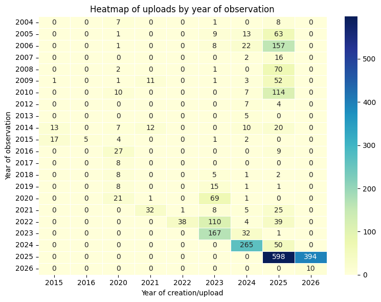

Now that is nice!

Uploads by iconic taxon

Next question was to visualise the relative number of records uploaded each year for different iconic taxon. I choose to use here a mosaic plot from package statsmodels. Each colum is a taxon, width is proportional to the number of records for the taxon, and the height of the segments of the columns represent the proportion of records for that taxon in each year.

plt.rcParams["figure.figsize"] = [9.00, 6.50]
plt.rcParams["figure.autolayout"] = True

def void_labelizer(key):
    key1, key2 = key
    return None

mosaic(df, ['iconic_taxon','year_uploaded'], 
       title='Mosaic Plot: iconic taxa per year', 
       horizontal=True, labelizer=void_labelizer,
       gap=0.005,
      label_rotation=[90.0,0])
plt.show()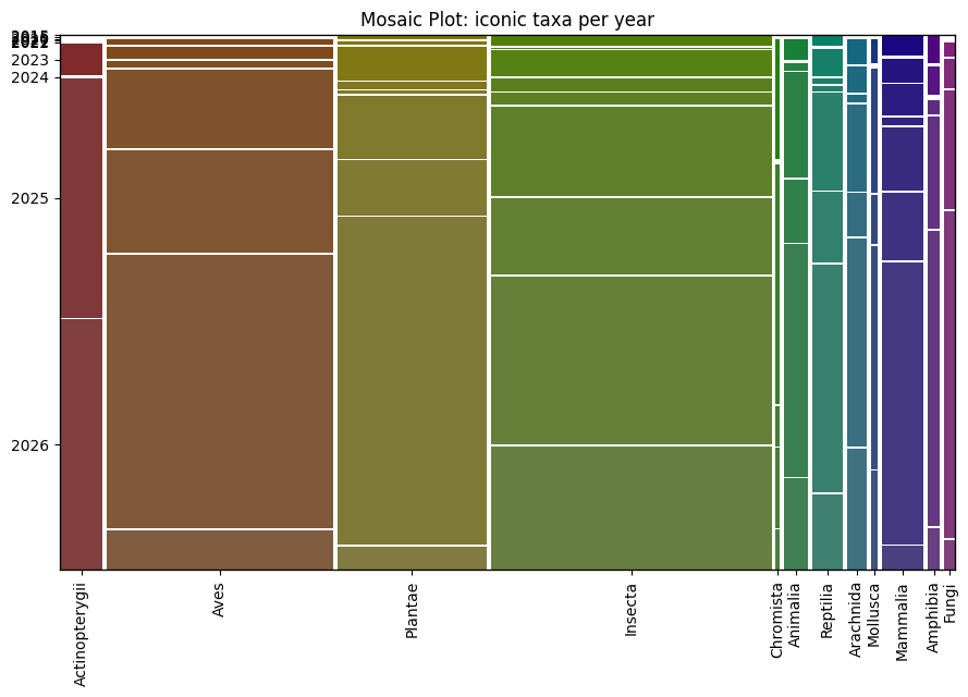

This plot shows a lot of things, for example that I like to watch insects more than anything else, or that more than half of my plants and fungi observations were uploaded in 2025, etc.

Cool!

Tools for record creation

Last question was about the tools that I use for creating records. So far I have used four different methods for this.

You can check these methods here:

Directly on the iNat website
Using the iNaturalist iPhone App
Using the iNaturalist (iNat Next) App
Directly from my python scripts using my very own NM-iNat app

Here I match the values in the app column of my data frame with the four methods mentioned above:

df['method'] = "Unknown"
df['method'] = df['method'].case_when([
    (df.app==0, "iNat website"),
    (df.app==3, "iNaturalist iPhone App"),
    (df.app==843, "iNat Next"),
    (df.app==904, "NM-iNat")])

I now I can group records created by year and method and count the number of records and the range of years of observations.

df.groupby(['year_uploaded', 'method']).agg({'year_observed': ['min','max','count']})

		year_observed
		min	max	count
year_uploaded	method
2015	iNat website	2009	2015	31
2016	iNat website	2015	2015	5
2020	iNat website	2004	2020	105
2021	iNat website	2009	2021	47
2021	iNaturalist iPhone App	2021	2021	9
2022	iNat website	2022	2022	19
2022	iNaturalist iPhone App	2021	2022	20
2023	iNat website	2004	2023	318
2023	iNaturalist iPhone App	2022	2023	77
2024	iNat website	2005	2024	315
2024	iNaturalist iPhone App	2020	2024	65
2025	NM-iNat	2005	2025	467
	iNat Next	2024	2025	54
	iNat website	2004	2025	686
	iNaturalist iPhone App	2024	2025	22
2026	NM-iNat	2025	2025	391
	iNat Next	2026	2026	10
	iNat website	2025	2025	3

My first uploads were all made using the iNat website, in this is still my preferred method for uploads. In 2021 I started to use iNaturalist iPhone App for some of my uploads. In 2025 I started to use the iNat Next version of the app, but I also started to use my own code to upload directly, and this is starting to become my favourite method.

Conclusion

This is it for now!

This post was all about dissecting my record creation history. I started with few manual uploads and have been growing my number of records in the last few years by going through my collection of old photographs and using different methods/tools for upload. Each year I organise myself better to discover those hidden gems of old observations. New tools help me to do this at ever increasing rate.

I hope you also enjoyed the graphics, and can use the code for your own projects.